
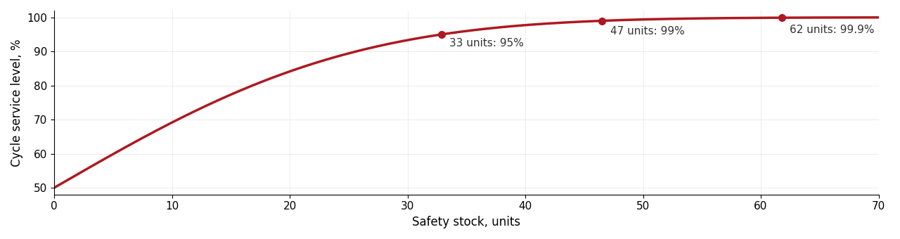
A good safety stock is the buffer above your forecast formed primarily by three things: how much structure your forecast captures correctly, how much variability is left after that, and what service level you target — plus the lead time and the distributional assumptions behind the calculation. In the simplest textbook case it reduces to a quantile of the assumed demand distribution: for normally distributed demand and a 95% cycle service level, roughly 1.64 standard deviations of the forecast error. But the assumptions behind that formula rarely hold in practice, which is why there is no universal number and no universal formula.
Many consultancies say “this depends on your situation and your product”, and they are not wrong. For example, safety stock for intermittent demand relies on a very different set of assumptions than for the regular one. However, although the specific value depends on many factors, the following five elements will impact it no matter what:
- The forecast for the product;
- The variability of sales;
- The target cycle service level;
- The lead time;
- The assumed demand distribution.
Here is the breakdown of each one of those:
(1). The forecast corresponds to the structure we managed to capture in sales: whether there is a trend and/or seasonality in the data, whether there are promotions that impact the sales and/or competitors’ actions — all of these things form the structure, something that we can explain and extrapolate. If you get it wrong, you might miss the target substantially (e.g. under forecast), incurring high costs where it is completely unnecessary.
(2). The variability of sales comes down to capturing the size of the unexplainable part of your data, i.e. what is left after we capture as much structure as we can. This part corresponds to the fundamentally unpredictable information, e.g. whether an additional customer will come to our restaurant to order pepperoni pizza. If your forecast is wrong, the structure that you missed will be captured by the model as “noise”, and it will inflate the safety stock level, meaning that you will overstock.
(3). The target service level determines the percentage of demand you want to satisfy. Here we focus on the cycle service level (sometimes called P1): the probability of not running out of stock during a replenishment cycle. A 95% cycle service level means that on average in 95 out of 100 cycles you expect to satisfy all the demand, and in the remaining 5 you accept a stockout. It is not possible to satisfy everyone all the time, so we always keep in mind that in some cases customers will not be able to buy our product, and that’s totally fine. It might seem that setting the target to 99.99% is the best solution, because this way we avoid almost all stockouts. But safety stock grows non-linearly as the service level approaches 100%, so those last fractions of a percent cost much more than the ones closer to 90%. In reality, the target service level should be defined based on the holding costs and lost sales: if your product is large and expensive and is bought only once per month, there’s no point in having hundreds of units on the shelves just in case lots of customers come one day to buy it. Decreasing the service level for such products can be a sensible strategy.
An important note! There is another measure whose definition sounds similar to the cycle service level: the fill rate (P2), the percentage of demand satisfied directly from stock. The two answer different questions — the cycle service level only cares whether the stockout happened or not, while the fill rate counts the units you failed to deliver. A cycle with one lost unit and a cycle with a hundred lost units are equally “failed” cycles for P1, but very different for P2. As a result, a 95% cycle service level and a 95% fill rate lead to very different safety stocks. Most textbook formulas, including the one below, assume the cycle service level, so make sure you know which of the two your company actually reports.
(4). Lead time is the time between placing a replenishment order and having the product available on the shelf (or usable in the warehouse). The longer the lead time is, the higher the uncertainty about the demand is, and thus the higher the safety stock becomes. By nature it is stochastic because there are many factors impacting when the product will be delivered, but many textbooks simplify this by using the average lead time instead of the real one. This leads to the potential underestimation of the uncertainty.
(5). The assumed distribution. The conventional textbook formula that you might have seen (Safety Stock = \(z \times \sigma \times \sqrt{L} \)) assumes independent identically distributed (i.i.d.) demand, following Normal distribution, which does not happen in real life often (if at all). The “i.i.d.” part of the equation is wrong because the demand on a weekday differs from the demand on the weekend, while the normality only holds asymptotically for high volume products. If you have intermittent demand, forget about Normality – this is not the case. Making wrong distributional assumptions leads to a safety stock that has nothing to do with reality, leading to increased costs.
Connecting these five elements gives us the “good amount of safety stock”. For a very general simplified example, when we sell thousands of units of a product monthly, where the normal distribution of demand can work as a potential approximation, setting the lead time to 1, and a cycle service level to 95%, we get:
\begin{equation}
\mathrm{Safety Stock}_t = 1.64 s_t ,
\end{equation}
where \(s_t\) is the standard deviation of the forecast error, and 1.64 is the 95% quantile of the standard normal distribution. The safety stock sits on top of the forecast: the level you order up to is
\begin{equation}
\mathrm{Order Up To}_t = F_t + 1.64 s_t .
\end{equation}
Note that there are many potential issues with these formulae, so they should not be applied universally — they only work in very narrow cases.
An example
To see how these elements interact, take a deliberately simplified case — a fast-moving product where the normal approximation from element (5) is defensible. Suppose the forecast is 100 units per week, the standard deviation of the forecast error is 20 units, the lead time is one week, and you target a 95% cycle service level. Then the safety stock is \(1.64 \times 20 \approx 33\) units, and you would order up to \(100 + 33 = 133\) units. Raise the target to 99%, and the safety stock jumps to \(2.33 \times 20 \approx 47\) units — a 14-unit increase for four percentage points. Push it to 99.9% and you need \(3.09 \times 20 \approx 62\) units. This is the non-linearity mentioned above: the closer to 100%, the more each additional fraction of a percent costs you in stock. Note however that in reality the orders are done in pallets, not in units, so practically speaking 95% and 99% might not matter if your orders are placed in 50 units. This is where theory meets practice — and it is exactly the kind of decision we help companies make. Contact us.