2.2 Law of Large Numbers and Central Limit Theorem
Consider a case, when you want to understand what is the average height of teenagers living in your town. It is very expensive and time consuming to go from one house to another and ask every single teenager (if you find one), what their hight is. If we could do that, we would get the true mean, true average height of teenagers living in the town. But in reality, it is more practical to ask a sample of teenagers and make conclusions about the “population” (all teenagers in the town) based on this sample. Indeed, you will spend much less time collecting the information about the height of 100 people rather than 100,000. However, when we take a sample of something, the statistics we work with will always differ from the truth: sample mean will never be equal to the true mean, but it can be shown mathematically that it will converge to the truth, when some specific conditions are met and when the sample size increases. If we set up the experiment correctly, then we can expect our statistics to follow some laws.
2.2.1 Law of Large Numbers
The first law is called the Law of Large Numbers (LLN). It is the theorem saying that (under wide conditions) the average of a variable obtained over the large number of trials will be close to its expected value and will get closer to it with the increase of the sample size. This can be demonstrated with the following example:
obs <- 10000
# Generate data from normal distribution
y <- rnorm(obs,100,100)
# Create sub-samples of 50 and 100 observations
y30 <- sample(y, 30)
y1000 <- sample(y, 1000)
par(mfcol=c(1,2))
hist(y30, xlab="y")
abline(v=mean(y30), col="red")
hist(y1000, xlab="y")
abline(v=mean(y1000), col="red")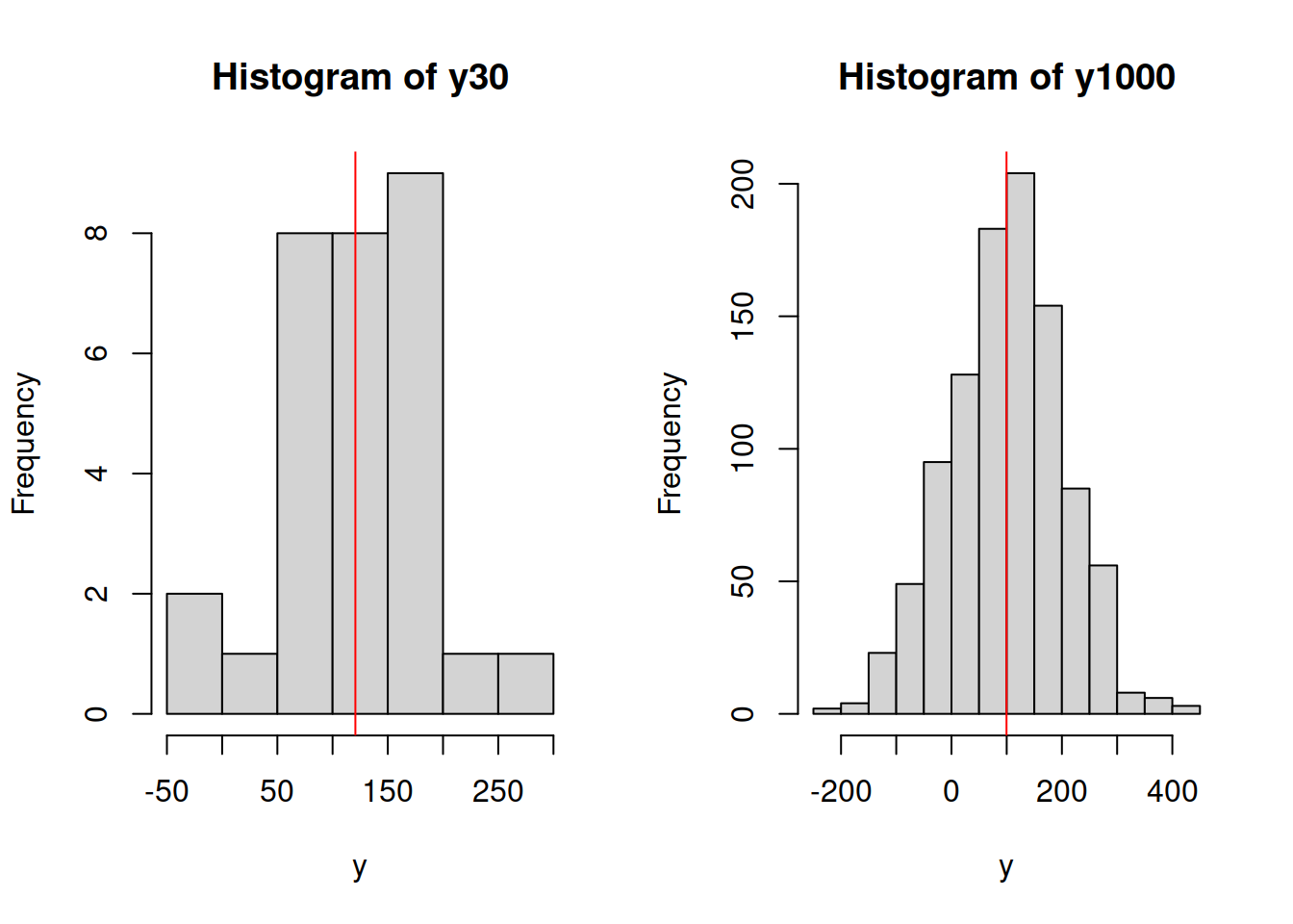
Figure 2.17: Histograms of samples of data from variable y.
What we will typically see on the plots above is that the mean (red line) on the left plot will be further away from the true mean of 100 than in the case of the right plot. Given that this is randomly generated, the situation might differ, but the idea would be that with the increase of the sample size the estimated sample mean will converge to the true one. We can even produce a plot showing how this happens:
yMean <- vector("numeric",obs)
for(i in 1:obs){
    yMean[i] <- mean(sample(y,i))
}
plot(yMean, type="l", xlab="Sample size", ylab="Sample mean")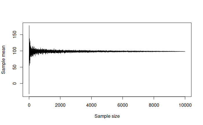
Figure 2.18: Demonstration of Law of Large Numbers.
We can see from the plot above that with the increase of the sample size the sample mean reaches the true value of 100. This is a graphical demonstration of the Law of Large Numbers: it only tells us about what will happen when the sample size increases. But it is still useful, because it used for many statistical inferences and if it does not work, then the estimate of mean would be incorrect, meaning that we cannot make conclusions about the behaviour in population.
In order for LLN to work, the distribution of variable needs to have finite mean and variance. This is discussed in some detail in the next subsection.
In summary, what LLN tells us is that if we average things out over a large number of observations, then that average starts looking very similar to the population value. However, this does not say anything about the performance of estimators on small samples.
2.2.2 Central Limit Theorem
As we have already seen on Figure 2.18, the sample mean is not exactly equal to the population mean even when the sample size is very large (thousands of observations). There is always some sort of variability around the population mean. In order to understand how this variability looks like, we could conduct a simple experiment. We could take a random sample of, for instance, 1000 observations several times and record each of the obtained means. We then can see how the variable will be distributed to see if there are any patterns in the behaviour of the estimator:
nIterations <- 1000
yMean <- vector("numeric",nIterations)
for(i in 1:nIterations){
    yMean[i] <- mean(sample(y,1000))
}
hist(yMean, xlab="Sample mean", main="")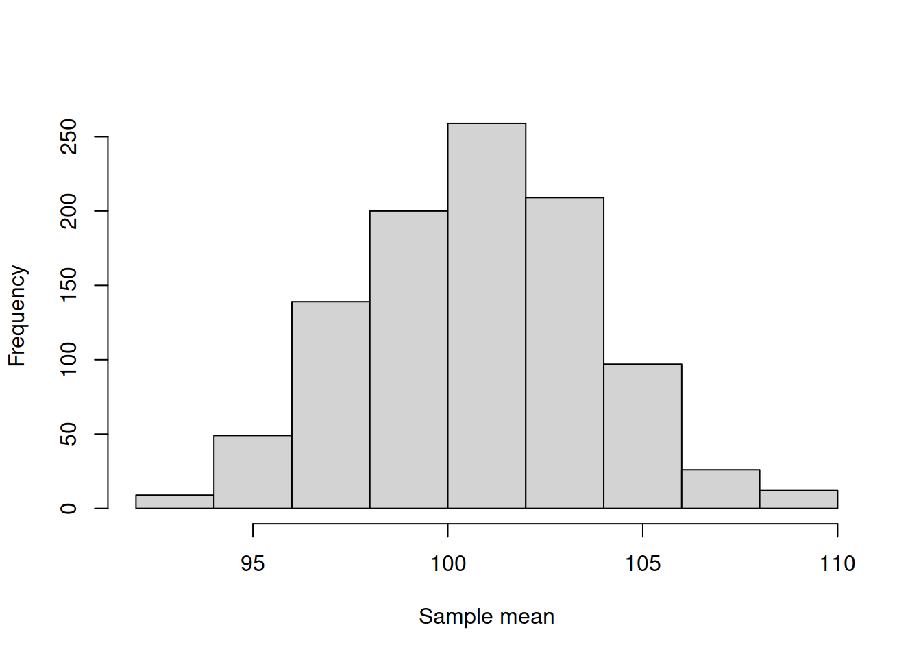
Figure 2.19: Histogram of the mean of the variable y.
There is a theorem that says that the distribution of mean in the experiment above will follow normal distribution under several conditions (discussed later in this section). It is called Central Limit Theorem (CLT) and very roughly it says that when independent random variables are added, their normalised sum will asymptotically follow normal distribution, even if the original variables do not follow it. Note that this is the theorem about what happens with the estimate (sum in this case), not with individual observations. This means that the error term might follow, for example, Inverse Gaussian distribution, but the estimate of its mean (under some conditions) will follow normal distribution. There are different versions of this theorem, built with different assumptions with respect to the random variable and the estimation procedure, but we do not dicuss these details in this textbook.
In order for CLT to hold, the following important assumptions need to be satisfied:
- The true value of parameter is not near the bound. e.g. if the variable follows uniform distribution on (0, \(a\)) and we want to estimate \(a\), then its distribution will not be Normal (because in this case the true value is always approached from below). This assumption is important in our context, because ETS and ARIMA typically have restrictions on their parameters.
- The random variables are identically independent distributed (i.i.d.). If they are not, then their average might not follow normal distribution (in some conditions it still might).
- The mean and variance of the distribution are finite. This might seem as a weird issue, but some distributions do not have finite moments, so the CLT will not hold if a variable follows them, just because the sample mean will be all over the plane due to randomness and will not converge to the “true” value. Cauchy distribution is one of such examples.
If these assumptions hold, then CLT will work for the estimate of a parameter, no matter what the distribution of the random variable is. This becomes especially useful, when we want to test a hypothesis or construct a confidence interval for an estimate of a parameter.