Chapter 14 Model diagnostics
In this chapter, we investigate how ADAM can be diagnosed and improved. Most topics will build upon the typical model assumptions discussed in Subsection 1.4.1 and in Chapter 15 of Svetunkov and Yusupova (2025). Some of the assumptions cannot be diagnosed properly, but there are well-established instruments for others. All the assumptions about statistical models can be summarised as follows:
- Model is correctly specified:
- Residuals are i.i.d.:
- They are not autocorrelated;
- They are homoscedastic;
- The expectation of residuals is zero, no matter what;
- The residuals follow the specified distribution;
- The distribution of residuals does not change over time.
- The explanatory variables are not correlated with anything but the response variable:
- No multicollinearity;
- No endogeneity (not discussed in the context of ADAM).
Technically speaking, (3) is not an assumption about the model, it is just a requirement for the estimation to work correctly. In regression context, the satisfaction of these assumptions implies that the estimates of parameters are efficient and unbiased (respectively for (3a) and (3b)).
In general, all model diagnostics are aimed at spotting patterns in residuals. If there are patterns, then some assumption is violated and something is probably missing in the model. In this chapter, we will discuss which instruments can be used to diagnose different types of violations of assumptions.
Remark. The analysis carried out in this chapter is based mainly on visual inspection of various plots. While there are statistical tests for some assumptions, we do not discuss them here. This is because in many cases human judgment is at least as good as automated procedures (Petropoulos et al., 2018b), and people tend to misuse the latter (Wasserstein and Lazar, 2016). So, if you can spend time on improving the model for a specific data, the visual inspection will typically suffice.
To make this more actionable, we will consider a conventional regression model on Seatbelts data, discussed in Section 10.6. We start with a pure regression model, which can be estimated equally well with the adam() function from the smooth package or the alm() from the greybox in R. In general, I recommend using alm() when no dynamic elements are present in the model (or only AR(p) and/or I(d) are needed). Otherwise, you should use adam() in the following way:
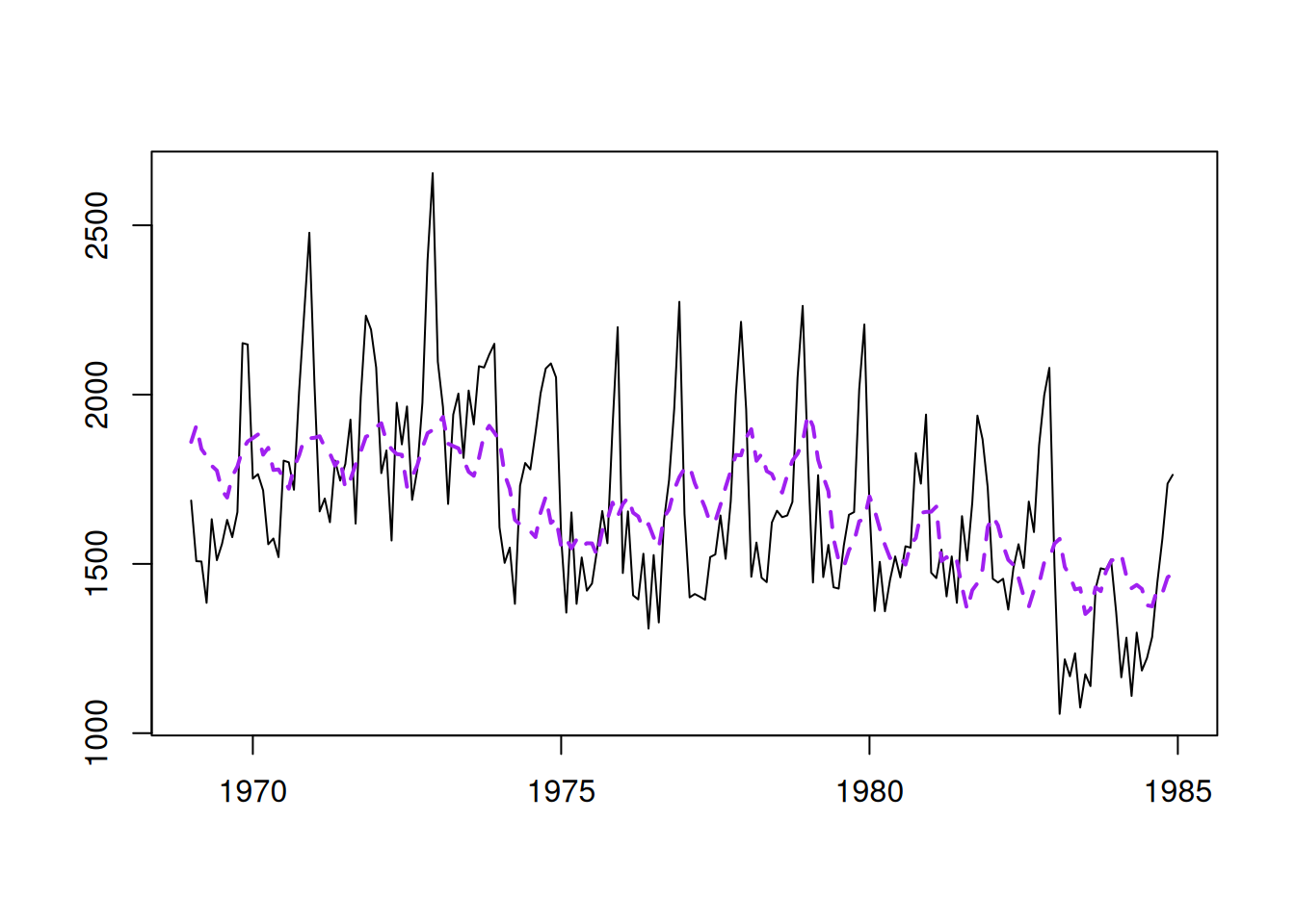
Figure 14.1: Basic regression model for the data on road casualties in Great Britain 1969–1984.
This model has several issues, and in this chapter, we will discuss how to diagnose and fix them.