13.4 Examples of application
We consider the same example from Section 13.1. Just as a reminder, in that example, both demand occurrence and demand sizes increase over time (Figure 13.1), meaning that we can try the model with the trend for both parts. This can be done using the adam() function from the smooth package, defining the type of occurrence to use. We will try several options and select the one that has the lowest AICc:
adamiETSy <- vector("list",4)
adamiETSy[[1]] <- adam(y, "MMdN", h=10, holdout=TRUE,
                       occurrence="odds-ratio")
adamiETSy[[2]] <- adam(y, "MMdN", h=10, holdout=TRUE,
                       occurrence="inverse-odds-ratio")
adamiETSy[[3]] <- adam(y, "MMdN", h=10, holdout=TRUE,
                       occurrence="direct")
adamiETSy[[4]] <- adam(y, "MMdN", h=10, holdout=TRUE,
                       occurrence="general")
adamiETSyAICcs <-
    setNames(sapply(adamiETSy,AICc),
             c("odds-ratio", "inverse-odds-ratio",
               "direct", "general"))
adamiETSyAICcs
## odds-ratio inverse-odds-ratio direct general
## 398.3674 407.5351 395.4822 398.3975Based on this, we can see that the model with direct probability has the lowest AICc. We can show how the model approximates the data and produces forecasts for the holdout:
i <- which.min(adamiETSyAICcs)
par(mfcol=c(2,1), mar=c(2,2,2,1))
plot(adamiETSy[[i]],7)
plot(adamiETSy[[i]]$occurrence,7)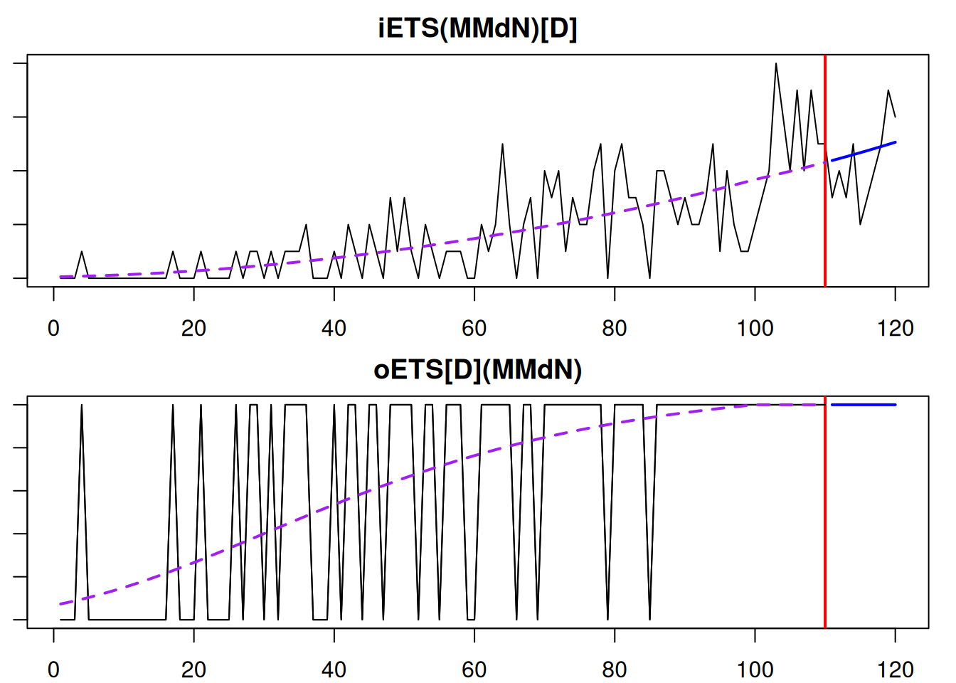
Figure 13.9: The fit of the best model to the intermittent data: final demand and the demand occurrence parts.
Figure 13.9 shows that the model captured the trend well for both the demand occurrence and demand sizes parts. It forecasts that the mean demand will increase for the holdout period. We can also explore the demand occurrence part of this model by typing:
## Occurrence model
## Time elapsed: 0.02 seconds
## Model estimated using om() function: oETS(MMdN)[D]
## With backcasting initialisation
## Distribution assumed in the model: Cumulative Logistic
## Loss function type: likelihood; Loss function value: 57.5726
## Persistence vector g:
##  alpha   beta
## 0.0986 0.0000
## Damping parameter: 0.1249
## Sample size: 110
## Number of estimated parameters: 5
## Number of degrees of freedom: 105
## Information criteria:
##      AIC     AICc      BIC     BICc
## 125.1452 125.7221 138.6476 140.0035
##
## Forecast errors:
## Asymmetry: 100%; sMSE: 0.058%; rRMSE: Inf; sPIS: -133.017%; sCE: 24.185%
In our example, the smoothing parameters are equal to zero for the demand occurrence part, which makes sense because the selected model is the damped multiplicative trend one, which should capture the increasing probability of occurrence well.
Depending on the generated data, there might be issues in the ETS(M,Md,N) model for demand sizes, if the smoothing parameters are too big, especially for the trend component. So, we can also try out the logARIMA(1,1,2) to see how it compares with this model. Given that ARIMA is not yet implemented for the occurrence part of the model, we need to construct the oETS separately and then use in adam():
oETSModel <- oes(y, "MMdN", h=10, holdout=TRUE,
                 occurrence=names(adamiETSyAICcs)[i])
adamiARIMA <- adam(y, "NNN", h=10, holdout=TRUE,
                   occurrence=oETSModel,
                   orders=c(1,1,2),
                   distribution="dlnorm")
adamiARIMA
## Time elapsed: 0.14 seconds
## Model estimated using adam() function: iARIMA(1,1,2)[D]
## With backcasting initialisation
## Occurrence model type: Direct
## Distribution assumed in the model: Mixture of Bernoulli and Log-Normal
## Loss function type: likelihood; Loss function value: 133.3548
## ARMA parameters of the model:
## Lag 1
## AR(1) -0.4046
## Lag 1
## MA(1) -0.2814
## MA(2) -0.4436
##
## Sample size: 110
## Number of estimated parameters: 6
## Number of degrees of freedom: 104
## Number of provided parameters: 5
## Information criteria:
## AIC AICc BIC BICc
## 393.8548 394.6703 410.0576 411.9743
##
## Forecast errors:
## Asymmetry: 45.292%; sMSE: 55.286%; rRMSE: 0.972; sPIS: -2040.157%; sCE: 298.239%Comparing the iARIMA model with the previous iETS based on AICc would not be fair because as soon as the occurrence model is provided to the adam(), it does not count the parameters estimated in that part towards the overall number of estimated parameters. To make the comparison fair, we need to make ADAM iETS comparable by estimating it in a similar way:
## Time elapsed: 0.06 seconds
## Model estimated using adam() function: iETS(MMdN)[D]
## With backcasting initialisation
## Occurrence model type: Direct
## Distribution assumed in the model: Mixture of Bernoulli and Gamma
## Loss function type: likelihood; Loss function value: 128.7607
## Persistence vector g:
## alpha  beta
## 0.006 0.006
## Damping parameter: 0.9933
## Sample size: 110
## Number of estimated parameters: 6
## Number of degrees of freedom: 104
## Number of provided parameters: 5
## Information criteria:
##      AIC     AICc      BIC     BICc
## 384.6667 385.4822 400.8696 402.7863
##
## Forecast errors:
## Asymmetry: 2.365%; sMSE: 51.095%; rRMSE: 0.935; sPIS: -1009.348%; sCE: 51.131%
Comparing information criteria, the iETS model is more appropriate for this data. But this might be due to different distributional assumptions and difficulties estimating the ARIMA model. If you want to experiment more with iARIMA, you might try fine tuning its parameters (see Section 11.4.1) for the data either by increasing the maxeval or changing the initialisation, for example:
adamiARIMA <- adam(y, "NNN", h=10, holdout=TRUE,
                   occurrence=oETSModel, orders=c(1,1,2),
                   distribution="dgamma", initial="back")
Finally, we can produce point and interval forecasts from either of the models via the forecast() method. Here is an example:
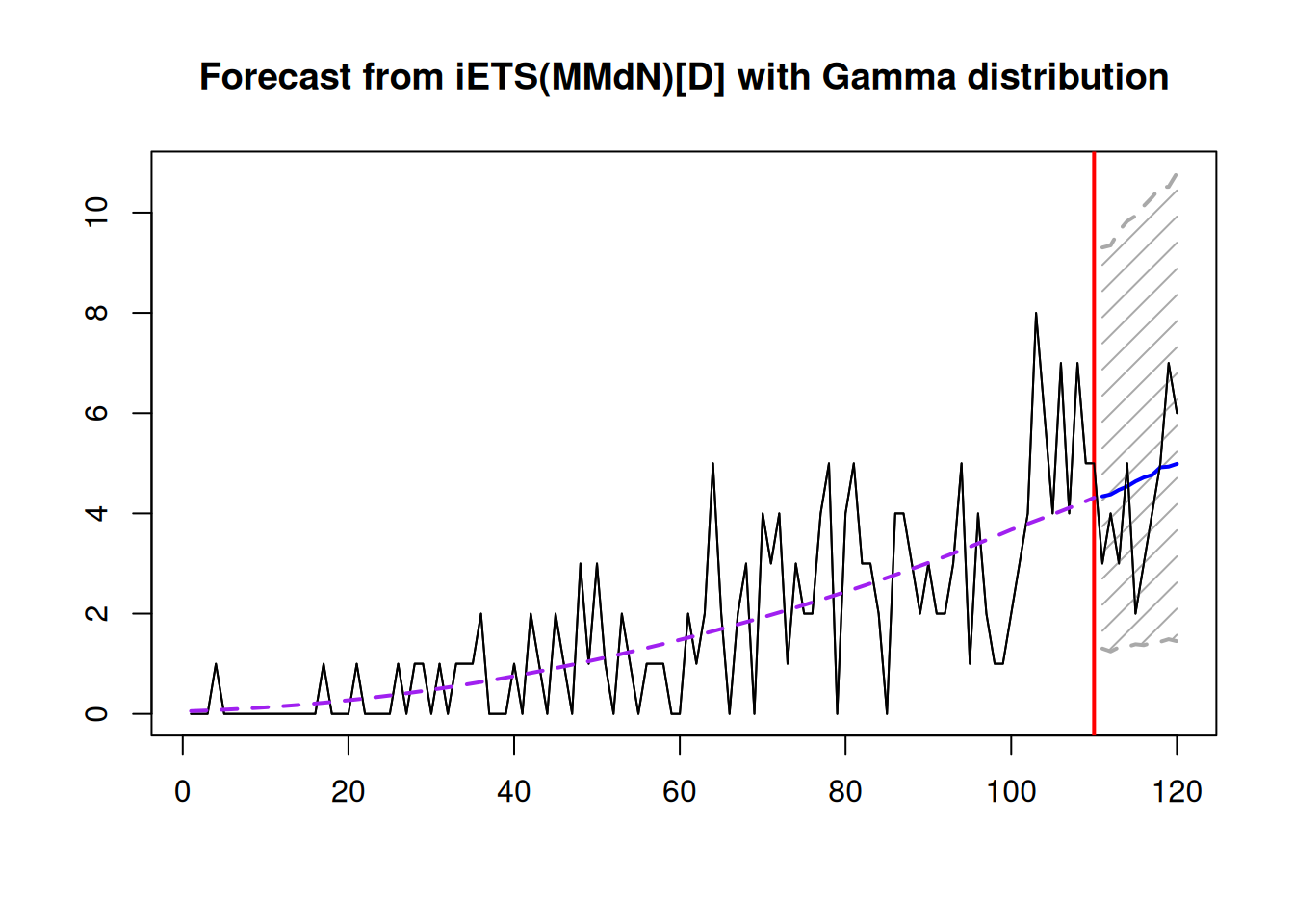
Figure 13.10: Point forecasts and prediction interval from the iETS(M,Md,N)\(_D\) model.
In Figure 13.10, the interval is expanding, reflecting the captured tendency of growth in the data. The prediction interval produced from multiplicative ETS models will typically be simulated if interval="prediction", so to make them smoother, you might need to increase the nsim parameter, for example, to nsim=100000.
The software behind this book. The methods described here are implemented in the smooth and greybox packages for R and Python, which are free and open source.
Want to learn this with us? We teach these methods to practitioners on Demand Forecasting Principles, a four-week online course, and run other courses in forecasting, statistics and analytics.