18.1 Creating simulation paths
As mentioned earlier in previous chapters, for some models, the conditional \(h\) steps ahead moments do not have analytical expressions. For example, as discussed in Section 6.3, pure multiplicative models typically do not have formulae for the conditional expectations and variance for longer horizons. The one exception is the ETS(M,N,N) model, where the point forecast corresponds to the conditional expectation for any horizon as long as the expectation of the error term \(1+\epsilon_t\) is equal to one. This problem is not only important for the moments, but it also arises when quantiles of distributions are needed, especially for models with multiplicative error. In all these cases, when the moments and/or quantiles are not available analytically, they need to be obtained via other means. One of those is simulating many trajectories and then calculating moments numerically.
18.1.1 Simulating trajectories
The general idea of this approach is based on the discussion in Section 16.1: we use the estimated parameters, the last obtained state vector (level, trend, seasonal, ARIMA components, etc.) and the estimate of the scale of distribution to generate the possible paths of the data for the next \(h\) observations. The simulation itself is done in several steps:
- Generate \(h\) random variables for the error term, \(\epsilon_{t+j}\) or \(1+\epsilon_{t+j}\) – depending on the type of error, assumed distribution in the model (the latter was discussed in Sections 5.5 and 6.5), and estimated parameters of distribution (such as scale);
- Insert the error terms in the state space model (7.1) from Section 7.1, both in the transition and observation parts, do that iteratively from \(j=1\) to \(j=h\): \[\begin{equation*} \begin{aligned} {y}_{t+j} = &w(\mathbf{v}_{t+j-\boldsymbol{l}}) + r(\mathbf{v}_{t+j-\boldsymbol{l}}) \epsilon_{t+j} \\ \mathbf{v}_{t+j} = &f(\mathbf{v}_{t+j-\boldsymbol{l}}) + g(\mathbf{v}_{t+j-\boldsymbol{l}}) \epsilon_{t+j} \end{aligned}; \end{equation*}\]
- Record actual values for \(j=\{1, \dots, h\}\);
- Repeat (1) – (3) \(n\) times;
- Take desired moments or quantiles for each horizon from 1 to \(h\).
Graphically, the result of this approach is shown in Figure 18.1, where each separate path is shown in grey colour, and the expectation is in black. See the R code for this in Subsection 18.1.2.
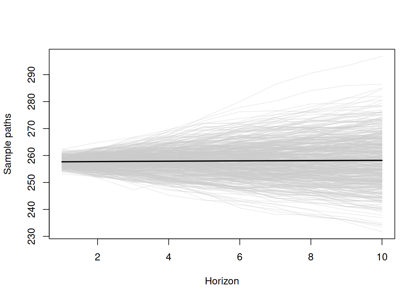
Figure 18.1: Sample paths (scenarios) generated from ADAM for the holdout sample.
Remark. In the case of multiplicative trend or multiplicative seasonality, it makes sense to take trimmed mean instead of the basic arithmetic one on step (5). This is because the models with these components might exhibit explosive behaviour, and thus the expectation might become unrealistic. I suggest using 1% trimming, although this does not have any scientific merit and is only based on my personal expertise.
The simulation-based approach is universal, no matter what model is used, and can be applied to any ETS, ARIMA, Regression model, or combination (including dynamic ETSX, intermittent demand, and multiple frequency models). Furthermore, instead of extracting moments on step five, one can take geometric mean, median, or any other desired statistics.
The main issue with this approach is that the conditional expectation, or any other statistics calculated based on this, will differ from one simulation run to another. If \(n\) is small, these values will be less stable (vary more with the new runs). But, with the increase of \(n\), they will reach some asymptotic values, staying random nonetheless. However, this is a good thing because this randomness reflects the uncertain nature of these statistics in the sample: the true values are never known, and the estimates will inevitably change with the sample size change. Another limitation is the computational time and memory usage: the more iterations we want to produce, the more calculations will need to be done, and more memory will be consumed. Luckily, time complexity in this situation is linear: \(O(h \times n)\).
18.1.2 Demonstration in R
In order to demonstrate the simulation approach, we consider an artificial case of an ETS(M,M,N) model with \(l_t=1000\), \(b_t=0.95\), \(\alpha=0.1\), \(\beta=0.01\), and Gamma distribution for error term with scale \(s=0.05\). We generate 1000 scenarios from this model for the horizon of \(h=10\) using the sim.es() function from the smooth package:
nsim <- 1000
h <- 10
s <- 0.1
initial <- c(1000,0.95)
persistence <- c(0.1,0.01)
y <- sim.es("MMN", obs=h, nsim=nsim, persistence=persistence,
            initial=initial, randomizer="rgamma",
            shape=1/s, scale=s)
After running the code above, we will obtain an object y that will contain several variables, including y$data with all the 1000 possible future trajectories. We can plot them to get an impression of what we are dealing with (see Figure 18.2):
plot(y$data[,1], ylab="Sales", ylim=range(y$data),
     col=rgb(0.8,0.8,0.8,0.4), xlab="Horizon")
# Plot all the generated lines
for(i in 2:nsim){
  lines(y$data[,i], col=rgb(0.8,0.8,0.8,0.4))
}
# Add conditional mean and quantiles
lines(apply(y$data,1,mean))
lines(apply(y$data,1,quantile,0.025),
      col="grey", lwd=2, lty=2)
lines(apply(y$data,1,quantile,0.975),
      col="grey", lwd=2, lty=2)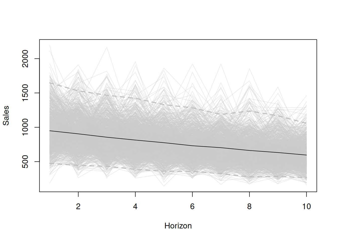
Figure 18.2: Data generated from 1000 ETS(M,M,N) models.
Based on the plot in Figure 18.2, we can see what the conditional \(h\) steps ahead expectation (black line) and what the 95% prediction interval will be for the data based on the ETS(M,M,N) model with the parameters mentioned above.
Similar paths are produced by the forecast() method for the adam class in the package smooth. If you need to extract them for further analysis, they are returned in the object scenarios if the parameters interval="simulated" and scenarios=TRUE are set.