18.4 Other aspects of forecast uncertainty
There are other elements related to forecasting and taking uncertainty into account that we have not discussed in the previous sections. Here we discuss several special cases where forecasting approaches might differ from the conventional ones.
18.4.1 Prediction interval for intermittent demand model
When it comes to constructing a prediction interval for the intermittent state space model (from Chapter 13), then there is an important aspect that should be taken into account. Given that the model consists of two parts: demand sizes and demand occurrence, the prediction interval should take the uncertainty from both of them into account. In this case, we should first predict the probability of occurrence of demand for the \(h\) steps ahead and then decide what the width of the interval should be based on this probability. For example, if we estimate that the demand will occur with probability \(\hat{p}_{t+h|t} = 0.8\), then this means that we expect that in 20% of the cases, we will observe zeroes. This should reduce the confidence level for the demand sizes. Formally speaking, this comes to the following equation: \[\begin{equation} F_{y_{t+h}}(y_{t+h} \leq q) = \hat{p}_{t+h|t} F_{z_{t+h}}(z_{t+h} \leq q) +(1 -\hat{p}_{t+h|t}), \tag{18.8} \end{equation}\] where \(F_{y_{t+h}}(\cdot)\) is the cumulative distribution function of demand, \(F_{z_{t+h}}(\cdot)\) is the cumulative distribution function of the demand sizes, \(\hat{p}_{t+h|t}\) is the \(h\) steps ahead expected probability of occurrence, and \(q\) is the quantile of distribution. In the formula (18.8), we know the expected probability and we know the confidence level \(F_{y_{t+h}}(y_{t+h} \leq q)\). The unknown element is the \(1-\alpha = F_{z_{t+h}}(z_{t+h} \leq q)\). So after regrouping elements we get: \[\begin{equation} F_{z_{t+h}}(z_{t+h} \leq q) = \frac{F_{y_{t+h}}(y_{t+h} \leq q) -(1 -\hat{p}_{t+h|t})}{\hat{p}_{t+h|t}}, \tag{18.9} \end{equation}\] which can be used for the calculation of the confidence level of a prediction interval. For example, if the confidence level is 0.95 and the expected probability of occurrence is 0.8, then \(F_{z_{t+h}}(z_{t+h} \leq q) = \frac{0.95 -0.2}{0.8} = 0.9375\). Assuming that demand sizes follow some distribution (e.g. Gamma), we can use formula (18.3) to construct a prediction interval of the width 93.75%, which will imply that 95% of demand is expected to be in the constructed bounds.
18.4.2 One-sided prediction interval
In some cases, we might not need both bounds of the interval. For example, when we deal with intermittent demand, we know that the lower bound will be equal to zero in many cases. Another example is the safety stock calculation: we only need the upper bound of the interval, and we need to make sure that the specific proportion of demand is satisfied (e.g. 95% of it). In these cases, we can just focus on the particular bound of the interval and drop the other one. Statistically speaking, this means that we cut only one tail of the assumed distribution.
Remark. In the case of an intermittent demand model, when the significance level is lower than the probability of inoccurrence \(1-p_{t+h|t}\), we will have the quantile equal to zero because the probability of having zeroes is higher than the significance level.
The one-sided interval has its implications and issues in several scenarios:
- When we are interested in the upper bound only and deal with positive distribution of demand (for example, Gamma, Log-Normal, or Inverse Gaussian), we know that the demand will always lie between zero and the constructed bound. In cases of low volume (or even intermittent) data, this makes sense because the original data might contain zeroes or have values close to it. The upper bound in this case will be lower than in the case of the two-sided prediction interval because we would not be splitting the probability into two parts (for the left and the right tails);
- The combination of the lower bound and positive distribution implies that the demand will be greater than the specified value in the pre-selected number of cases (defined by confidence level). There is no natural bound from above, so from a theoretical point of view, this implies that the demand can be infinite;
- The upper or lower bound with real-valued distribution (such as Normal, Laplace, S, or Generalised Normal) implies that the demand is either below or above the specified level, respectively, without any natural limit on the other side. If Normal distribution is used on positive low volume data, there is a natural lower bound, but the model itself will not be aware of it and will not restrict the space with the specific value, implying that the demand can be anything between the \(-\infty\) and the selected value.
From the practical point of view, the case with the upper bound and a positively defined distribution makes more sense than the other two cases, because if we are interested in demand forecasting, having a non-negative demand makes more sense than having a real-valued one, while the upper bound aligns better with a safety stock calculation.
18.4.3 Cumulative over the horizon forecast
Another related thing to consider when producing forecasts in practice is that the point forecast is not needed in some contexts. Instead, the cumulative over the forecast horizon (or over the lead time) might be more suitable. The classic example is the safety stock calculation based on the lead time (time between the order of a product and its delivery). In this situation, we need to make sure that while the product is being delivered, we do not run out of stock, thus still satisfying the selected level of demand (e.g. 95%), but now over the whole period of time rather than on every separate observation.
In the case of pure additive ADAM, there are analytical formulae for the conditional expectations and conditional variance for this case that can be used in forecasting. These formulae come directly from the recursive relation (5.10) (for derivations for a simpler case, see for example, Hyndman et al. (2008) and Svetunkov and Petropoulos (2018)): \[\begin{equation} \begin{aligned} \mu_{Y,t,h} = \text{E}(Y_{c,t,h}|t) = & \sum_{j=1}^h \sum_{i=1}^d \left(\mathbf{w}_{m_i}' \mathbf{F}_{m_i}^{\lceil\frac{j}{m_i}\rceil-1} \right) \mathbf{v}_{t} \\ \sigma^2_{Y,h} = \text{V}(Y_{c,t,h}|t) = & \left(1 + \sum_{k=1}^{h-1} \left(1+ (h-k) \sum_{i=1}^d \left(\mathbf{w}_{m_i}' \sum_{j=1}^{\lceil\frac{k}{m_i}\rceil-1} \mathbf{F}_{m_i}^{j-1} \mathbf{g}_{m_i} \mathbf{g}'_{m_i} (\mathbf{F}_{m_i}')^{j-1} \mathbf{w}_{m_i} \right) \right) \right) \sigma^2 \end{aligned}, \tag{18.10}\end{equation}\] where \(Y_{c,t,h}=\sum_{j=1}^h y_{t+j}\) is the cumulative actual value and all the other variables have been defined in Section 5.2. Based on the expectation and variance above, we can construct a prediction interval as discussed in Section 18.3.
In cases of multiplicative and mixed ADAM, there are no closed forms for the conditional expectation and variance. As a result, simulations similar to the one discussed in Section 18.1 are needed to produce all possible paths for the next \(h\) steps ahead. The main difference would be that before taking the expectation or quantiles, the paths would need to be aggregated over the forecast horizon \(h\). This approach, together with the idea of a one-sided prediction interval, can be directly used to calculate the safety stock over the lead time.
18.4.4 Example in R
For demonstration purposes, we consider an artificial intermittent demand example, similar to the one from Section 13.4:
For simplicity, we apply an iETS(M,Md,N) model with odds ratio occurrence:
adamiETSy <- adam(y, "MMdN", occurrence="odds-ratio",
                  h=7, holdout=TRUE)
plot(adamiETSy, 7, xlab="Time", ylab="Sales")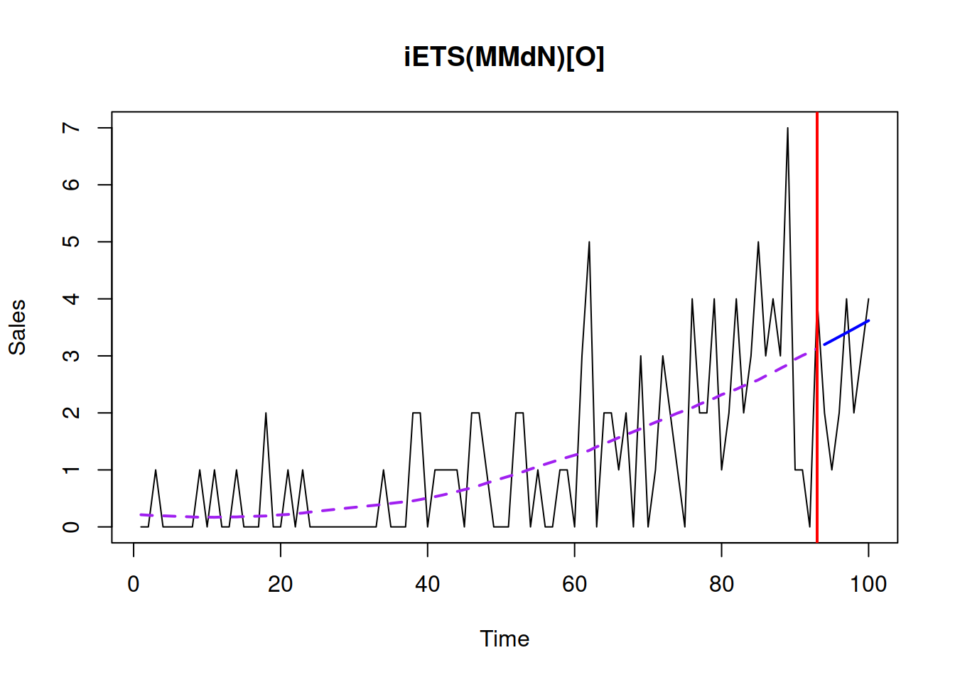
To make this setting closer to a possible real life situation, we assume that the lead time is seven days, and we need to satisfy the 99% of demand for the last seven observations based on our model. Thus we produce the upper bound for the cumulative values for the confidence level of 99%:
Given that we deal with cumulative values, the basic plot will not be helpful, and we should produce something different. Luckily, the plot() method for the ADAM forecasts take care of it. In the case of cumulative forecasts, it will aggregate the data to the same frequency as the forecast horizon and will produce the following plot (see Figure 18.8):
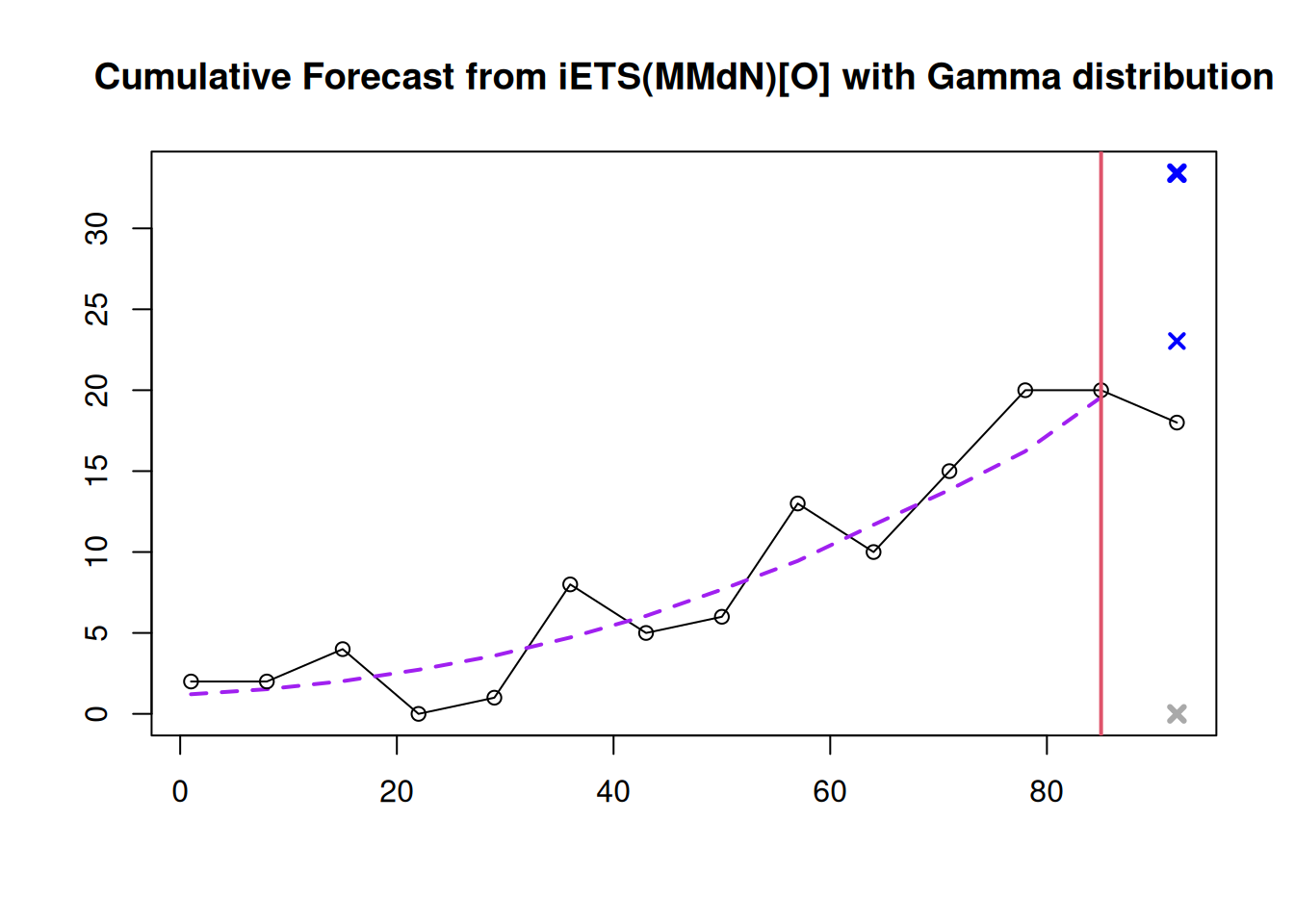
Figure 18.8: The actual cumulative demand (black line), the expectation (blue dot), and the 95% quantile of the distribution of the cumulative demand (the grey x) based on the iETS model.
What Figure 18.8 demonstrates is that for the holdout period of seven days, the cumulative demand was around 18 units, while the upper bound of the interval was approximately 33. Based on that upper bound, we could place an order (based on what we already have in stock) and have an appropriate safety stock.
This example is provided for demonstration purposes only. To see if the approach is suitable for a specific situation, we would need to apply it in either a rolling origin fashion (Section 2.4) or to a set of products to collect the distribution of related error measures.
18.4.5 Confidence interval
Finally, we can construct a confidence interval for some statistics. In general, it can be built for the mean, a parameter, fitted values, etc. In our context, we might be interested in the confidence interval for the conditional \(h\) steps ahead expectation. This implies that we are interested in the uncertainty of the line, not of the actual values, which can only be constructed for the model that takes the uncertainty of parameters into account (as discussed in Chapter 16). The construction of a confidence interval, in this case, relies on the Normal distribution (because of Central Limit Theorem), as long as the basic assumptions for the model and CLT are satisfied (see Section 6.2 and Chapter 15 of Svetunkov and Yusupova, 2025). Technically speaking, the construction of a confidence interval comes to capturing the model uncertainty discussed in Chapter 16.
18.4.5.1 Example in R
The only way that the confidence interval can be constructed for ADAM is via the reforecast() function. Consider the example with ADAM ETS(A,Ad,N) on BJSales data as in Section 18.3.8:
The confidence interval for this model can be produced either directly via reforecast() or via forecast(), which will call it for you:
Remark. I have increased the number of iterations for the simulation to get a more accurate confidence interval around the conditional expectation. This will consume more memory, as the operation involves creating 1000 sample paths for the fitted values and another 1000 for the holdout sample forecasts.
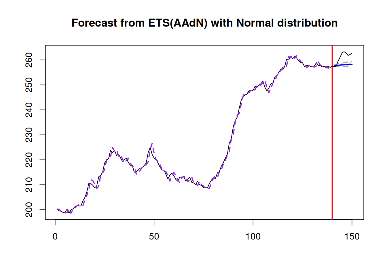
Figure 18.9: Confidence interval for the point forecast from an ADAM ETS(A,Ad,N) model.
Figure 18.9 shows the uncertainty around the point forecast based on the uncertainty of the parameters of the model. As can be seen, the interval is narrow, demonstrating that the conditional expectation would not change much if the model’s parameters would vary slightly. The fact that the actual values are systematically above the forecast does not mean anything because the confidence interval does not consider the uncertainty of actual values.