14.3 Model specification: Transformations
The question of appropriate transformations for variables in the model is challenging, because it is difficult to decide, what sort of transformation is needed, if needed at all. In many cases, this comes to selecting between an additive linear model and a multiplicative one. This implies that we compare the model: \[\begin{equation} y_t = a_0 + a_1 x_{1,t} + \dots + a_n x_{n,t} + \epsilon_t, \tag{14.1} \end{equation}\] with \[\begin{equation} y_t = \exp\left(a_0 + a_1 x_{1,t} + \dots + a_n x_{n,t} + \epsilon_t\right) . \tag{14.2} \end{equation}\] (14.2) is equivalent to the so called “log-linear” model, but can also include logarithms of explanatory variables instead of the variables themselves to become a “log-log” model. Fundamentally, the transformations of variables should be done based on the understanding of the problem rather than on technicalities.
There are different ways of diagnosing the problem with wrong transformations. The first one is the actuals vs fitted plot (Figure 14.7):
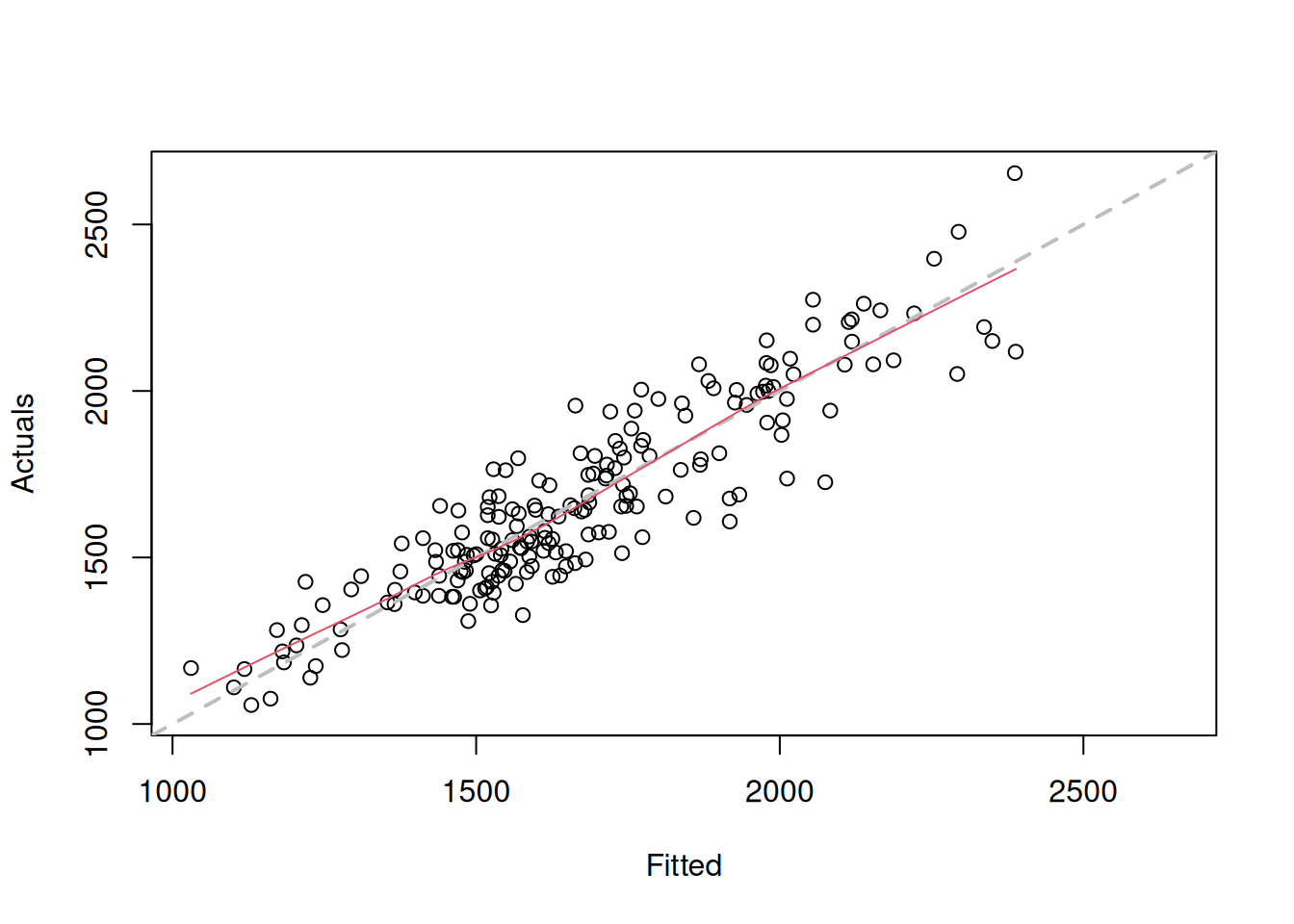
Figure 14.7: Actuals vs fitted for Model 3.
The grey dashed line on the plot in Figure 14.7 corresponds to the situation when actuals and fitted coincide (100% fit). The red line on the plot is the LOWESS line (Cleveland, 1979), produced by the LOWESS() function in R, smoothing the scatterplot to reflect the potential tendencies in the data. This red line should coincide with the grey line in the ideal situation. In addition, the variability around the line should not change with the increase of fitted values. In our case, there is a slight U-shape in the red line and a slight rise in variability around the middle of the data. This could either be due to pure randomness and thus should be ignored or indicate a slight non-linearity in the data. After all, we have constructed a pure additive model on the data that exhibits seasonality with multiplicative characteristics, which becomes especially apparent at the end of the series, where the drop in level is accompanied by the decrease of the variability of the data (Figure 14.8):
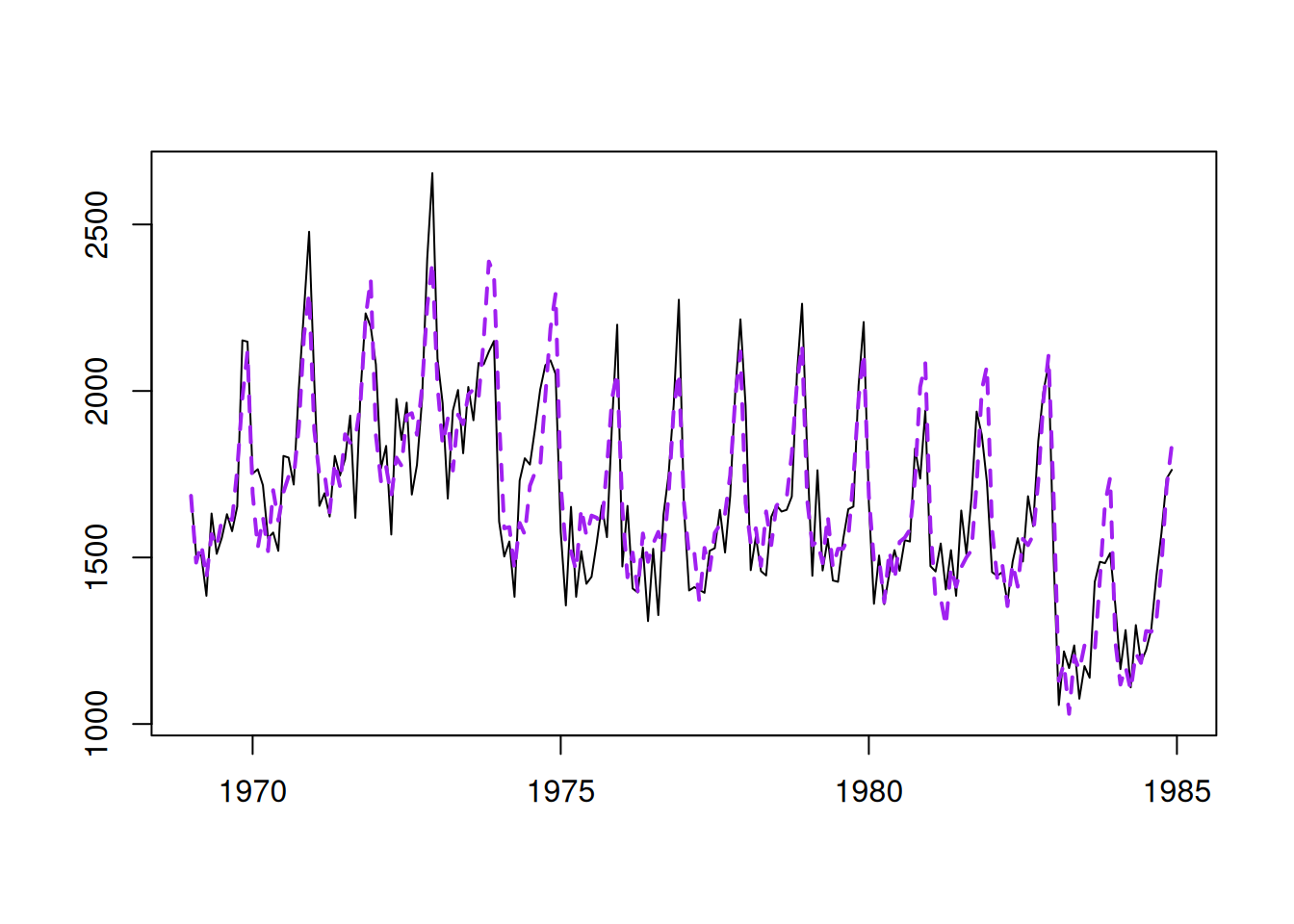
Figure 14.8: Actuals and fitted values for Model 3.
To diagnose this properly, we might use other instruments. One of these is the analysis of standardised residuals. The formula for the standardised residuals \(u_t\) will differ depending on the assumed distribution. For some of them it comes to the value inside the “\(\exp\)” part of the Probability Density Function:
- Normal, \(\epsilon_t \sim \mathcal{N}(0, \sigma^2)\): \(u_t = \frac{e_t -\bar{e}}{\hat{\sigma}}\);
- Laplace, \(\epsilon_t \sim \mathcal{Laplace}(0, s)\): \(u_t = \frac{e_t -\bar{e}}{\hat{s}}\);
- S, \(\epsilon_t \sim \mathcal{S}(0, s)\): \(u_t = \frac{e_t -\bar{e}}{\hat{s}^2}\);
- Generalised Normal, \(\epsilon_t \sim \mathcal{GN}(0, s, \beta)\): \(u_t = \frac{e_t -\bar{e}}{\hat{s}^{\frac{1}{\beta}}}\);
- Inverse Gaussian, \(1+\epsilon_t \sim \mathcal{IG}(1, \sigma^2)\): \(u_t = \frac{1+e_t}{\bar{e}}\);
- Gamma, \(1+\epsilon_t \sim \mathcal{\Gamma}(\sigma^{-2}, \sigma^2)\): \(u_t = \frac{1+e_t}{\bar{e}}\);
- Log Normal, \(1+\epsilon_t \sim \mathrm{log}\mathcal{N}\left(-\frac{\sigma^2}{2}, \sigma^2\right)\): \(u_t = \frac{e_t -\bar{e} +\frac{\hat{\sigma}^2}{2}}{\hat{\sigma}}\).
Here \(\bar{e}\) is the mean of residuals, which is typically assumed to be zero, and \(u_t\) is the value of standardised residuals. Note that the scales in the formulae above should be calculated via the formula with the bias correction, i.e. with the division by degrees of freedom, not the number of observations, otherwise the bias of scale might impact the standardised residuals. Also, note that in the cases of the Inverse Gaussian, Gamma, and Log-Normal distributions and the additive error, the formulae for the standardised residuals will be the same as shown above.
The standardised residuals can then be plotted against something else to do diagnostics of the model. Here is an example of a plot of fitted vs standardised residuals in R (Figure 14.9):
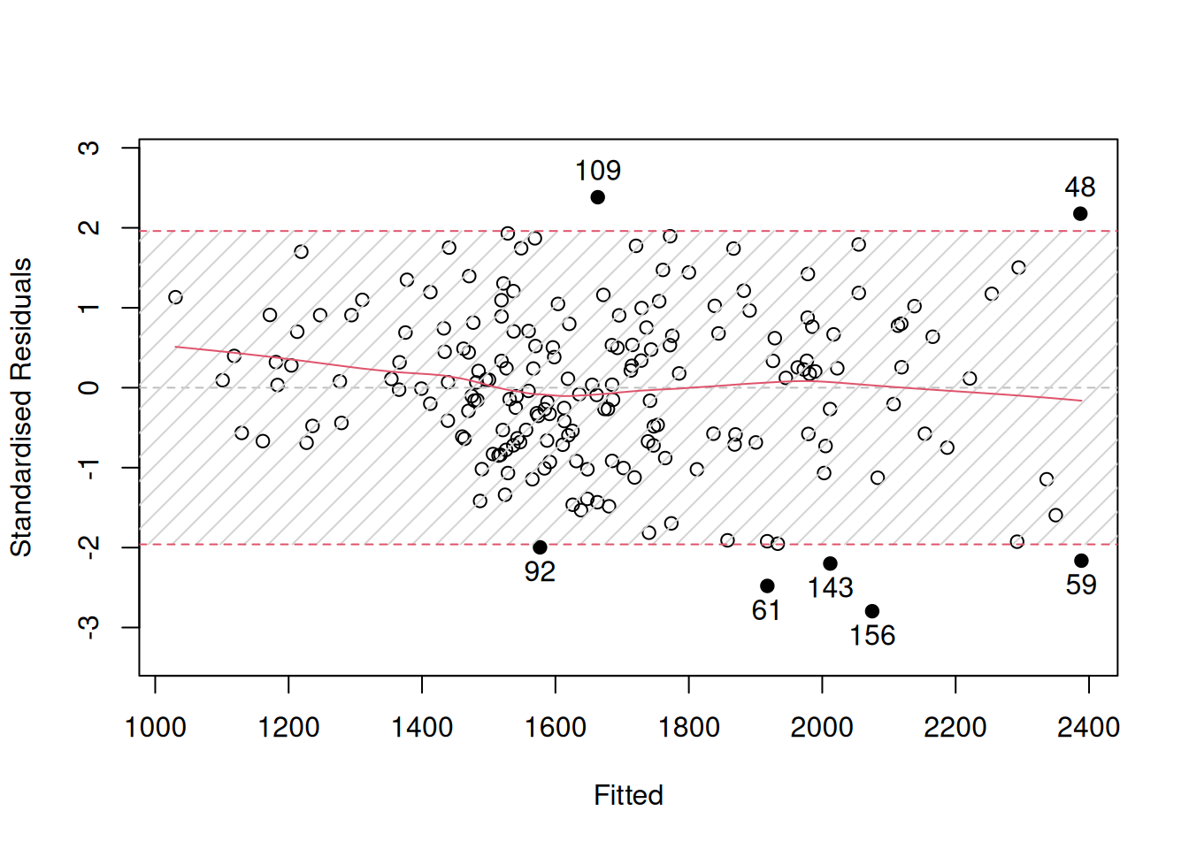
Figure 14.9: Standardised residuals vs fitted for a pure additive ETSX model.
Given that the scale of the original variable is now removed in the standardised residuals, it might be easier to spot the non-linearity. In our case, in Figure 14.9, it is still not apparent, but there is a slight curvature in the LOWESS line and a slight change in the variance: the variability in the beginning of the plot seems to be lower than the variability in the middle. Another plot that might be helpful (we have already used it before) is standardised residuals over time (Figure 14.10):
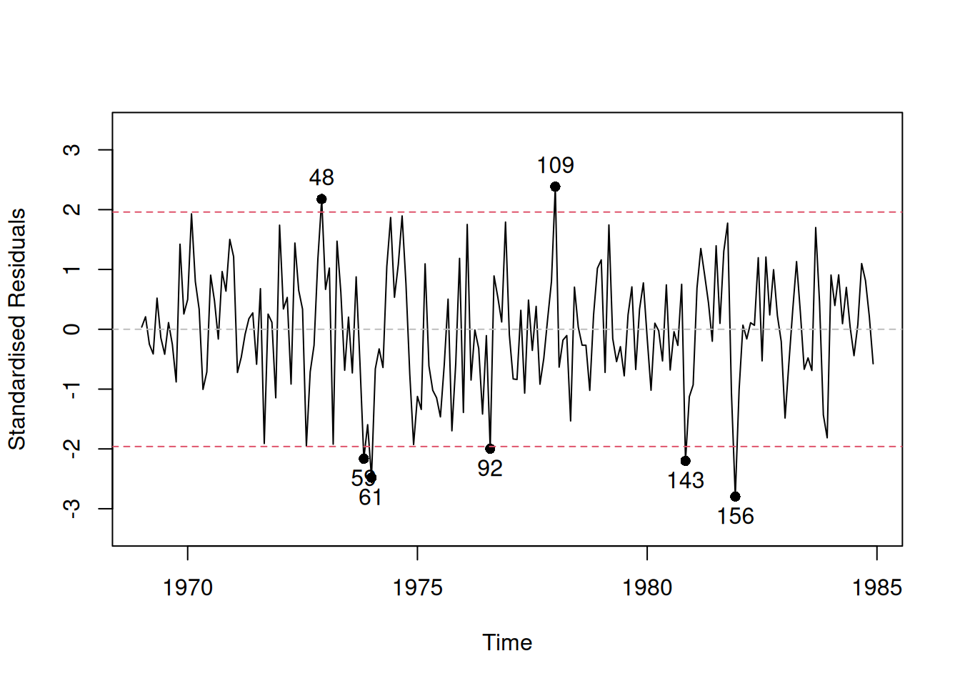
Figure 14.10: Standardised residuals vs time for a pure additive ETSX model.
The plot in Figure 14.10 does not show any apparent non-linearity in the residuals, so it is not clear whether any transformations are needed or not.
However, based on my judgment and understanding of the problem, I would expect the number of injuries and deaths to change proportionally to the change of the level of the data. If, after some external interventions, the overall level of injuries and deaths would decrease, then with a change of already existing variables in the model, we would expect a percentage decline, not a unit decline. This is why I will try a multiplicative model next (transforming explanatory variables as well):
adamSeat05 <- adam(Seatbelts, "MNM",
                   formula=drivers~log(PetrolPrice)+log(kms)+law)
plot(adamSeat05, 2, main="")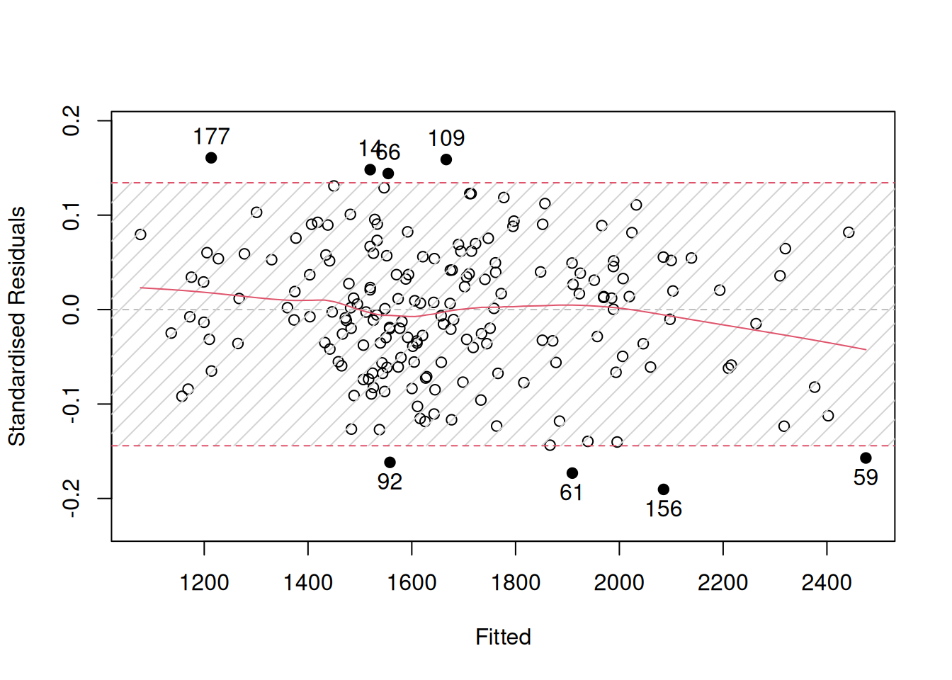
Figure 14.11: Standardised residuals vs fitted for a pure multiplicative ETSX model.
The plot in Figure 14.11 shows that the variability is now slightly more uniform across all fitted values, but the difference between Figures 14.9 and 14.11 is not very prominent. One of the potential ways of deciding what to choose in this situation is to compare the models using information criteria:
##       Additive model Multiplicative model
##             2401.736             2385.812
Based on this, we would be inclined to select the multiplicative model. My judgment in this specific case agrees with the information criterion.
We could also investigate the need for transformations of explanatory variables, but the interested reader is encouraged to do this analysis on their own.
Finally, the non-linear transformations are not limited with logarithm only. There are more of them, some of which are discussed in Chapter 14 of Svetunkov and Yusupova (2025).