13.1 Occurrence part of the model
The general model (13.1) assumes that demand occurs randomly and that the variable \(o_t\) can be either zero (no demand) or one (there is some demand). While this process can be modelled using different distributions, Svetunkov and Boylan (2023a) proposed using Bernoulli with a time varying probability: \[\begin{equation} o_t \sim \text{Bernoulli} \left(p_t \right) , \tag{13.2} \end{equation}\] where \(p_t\) is the probability of occurrence. The higher it is, the more frequently the demand will happen. If \(p_t=1\), then the demand becomes regular, while if \(p_t=0\), nobody buys the product at all. This section will discuss different types of models for the probability of occurrence. For each of them, there are different mechanisms of the model construction, estimation, error calculation, update of the states, and the generation of forecasts. To estimate any of these models, I recommend using likelihood, which can be calculated based on the Probability Mass Function (PMF) of Bernoulli distribution: \[\begin{equation} f_o(o_t, p_t) = p_t^{o_t}(1-p_t)^{1-o_t}. \tag{13.3} \end{equation}\] The parameters of the occurrence part of the model can be then estimated via the maximisation of the log-likelihood function, which comes directly from (13.3), and in the most general case is: \[\begin{equation} \ell \left(\boldsymbol{\theta}_o | \mathbf{o} \right) = \sum_{o_t=1} \log(\hat{p}_t) + \sum_{o_t=0} \log(1-\hat{p}_t) , \tag{13.4} \end{equation}\] where \(\hat{p}_t\) is the in-sample conditional one step ahead expectation of the probability on observation \(t\), given the information on observation \(t-1\), which depends on the vector of estimated parameters for the occurrence part of the model \(\boldsymbol{\theta}_o\).
In order to demonstrate the difference between specific types of oETS models, we will use the following artificial data:
Figure 13.1 shows how the data looks:
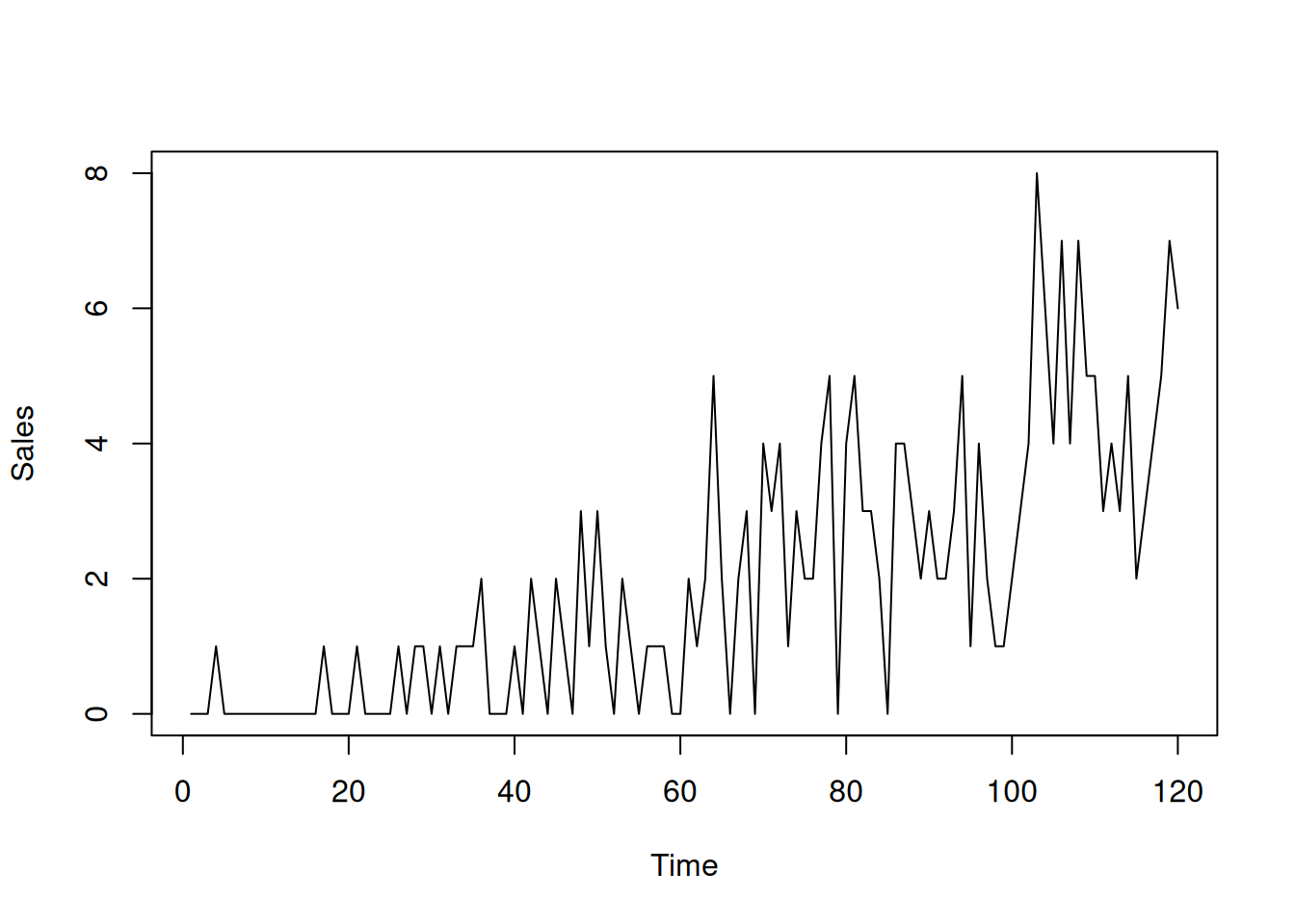
Figure 13.1: Example of intermittent demand data.
The probability of occurrence in this example increases together with the demand sizes. This example corresponds to the situation of intermittent demand for a product evolving to the regular one.
13.1.1 Fixed probability model, oETS\(_F\)
We start with the simplest case of fixed probability of occurrence, the oETS\(_F\) model: \[\begin{equation} o_t \sim \text{Bernoulli}(p) , \tag{13.5} \end{equation}\] This model assumes that demand happens with the same probability no matter what. This might sound exotic because, in practice, there might be many factors influencing customers’ desire to purchase, and the impact of these factors might change over time. But this is a basic model, which can be used as a benchmark on intermittent demand data. Furthermore, it might be suitable for modelling demand on expensive high-tech products, such as jet engines, which is “very slow” in its nature and typically does not evolve much over time.
When estimated via maximisation of the likelihood function (13.4), the probability of occurrence in this model is equal to: \[\begin{equation} \hat{p} = \frac{T_1}{T}, \tag{13.6} \end{equation}\] where \(T_1\) is the number of non-zero observations and \(T\) is the number of all the available observations in-sample.
The occurrence part of the model, oETS\(_F\) can be constructed using the oes() function from the smooth package:
## Occurrence state space model estimated: Fixed probability
## Underlying ETS model: oETS[F](MNN)
## Vector of initials:
##  level
## 0.6455
##
## Error standard deviation: 1.0909
## Sample size: 110
## Number of estimated parameters: 1
## Number of degrees of freedom: 109
## Information criteria:
##      AIC     AICc      BIC     BICc
## 145.0473 145.0844 147.7478 147.8349
The oETS\(_F\) model produces the straight line for the probability of 0.65, ignoring that in our example, the probability of occurrence has increased over time.
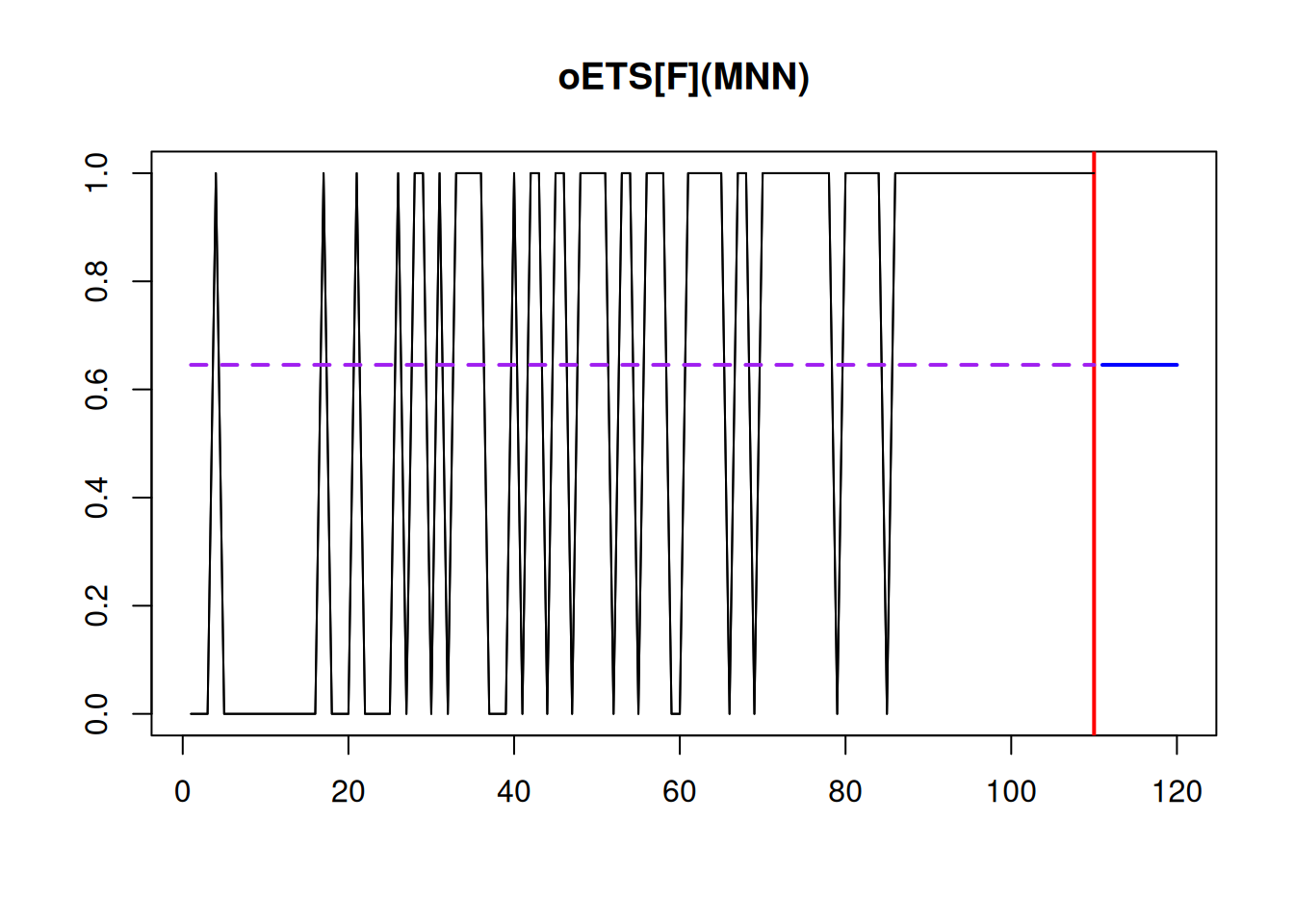
Figure 13.2: Demand occurrence and probability of occurrence in the oETS\(_F\) model.
The plot in Figure 13.2 demonstrates the dynamics of the occurrence variable \(o_t\) and the fitted and predicted probabilities. The solid line shows when zeroes and ones happen, depicting the variable \(o_t\). The dashed line corresponds to the fixed probability of occurrence \(\hat{p}\) in the sample.
13.1.2 Odds ratio model, oETS\(_O\)
In this model, it is assumed that the update of the probability is driven by the previously observed occurrence of a variable. It is more complicated than the previous model, as the probability now changes over time and can be modelled, for example, with an ETS(M,N,N) model: \[\begin{equation} \begin{aligned} & o_t \sim \text{Bernoulli} \left(p_t \right) \\ & p_t = \frac{\mu_{a,t}}{\mu_{a,t}+1} \\ & a_t = l_{a,t-1} \left(1 + \epsilon_{a,t} \right) \\ & l_{a,t} = l_{a,t-1}( 1 + \alpha_{a} \epsilon_{a,t}) \\ & \mu_{a,t} = l_{a,t-1} \end{aligned}, \tag{13.7} \end{equation}\] where \(l_{a,t}\) is the unobserved level component, \(\alpha_{a}\) is the smoothing parameter, \(1+\epsilon_{a,t}\) is the error term , which is positive, has the mean of one, and follows an unknown distribution, and \(\mu_{a,t}\)is the conditional expectation for the unobservable shape variable \(a_t\). The measurement and transition equations in (13.7) can be substituted by any other ETS, ARIMA, or regression model if it is reasonable to assume that the probability dynamic has some additional components, such as trend, seasonality, or exogenous variables. This model is called the “odds ratio” because the probability of occurrence in (13.7) is calculated using the classical logistic transform. This also means that \(\mu_{a,t}\) equals to: \[\begin{equation} \label{eq:oETS_O_oddsRatio} \mu_{a,t} = \frac{p_t}{1 -p_t} . \end{equation}\] When \(\mu_{a,t}\) increases in the oETS model, the odds ratio increases as well, meaning that the probability of occurrence goes up. Svetunkov and Boylan (2023a) explain that this model is, in theory, appropriate for the demand for products becoming obsolescent, because the multiplicative error ETS models asymptotically almost surely converge to zero. Still, given the updating mechanism, it should also work fine on other types of intermittent data.
When it comes to the application of the model to the data, its construction is done via the following set of equations (example with oETS\(_O\)(M,N,N)): \[\begin{equation} \begin{aligned} & \hat{p}_t = \frac{\hat{\mu}_{a,t}}{\hat{\mu}_{a,t}+1} \\ & \hat{\mu}_{a,t} = \hat{l}_{a,t-1} \\ & \hat{l}_{a,t} = \hat{l}_{a,t-1}( 1 + \hat{\alpha}_{a} e_{a,t}) \\ & 1+e_{a,t} = \frac{u_t}{1-u_t} \\ & u_{t} = \frac{1 + o_t -\hat{p}_t}{2} \end{aligned}, \tag{13.8} \end{equation}\] where \(e_{a,t}\) is the proxy for the unobservable error term \(\epsilon_{a,t}\) and \(\hat{\mu}_t\) is the estimate of \(\mu_{a,t}\). If a multiple steps ahead forecast for the probability is needed from this model, then the formulae discussed in Section 4.2 can be used to get \(\hat{\mu}_{a,t+h}\), which then can be inserted in the first equation of (13.8) to get the final conditional multiple steps ahead probability of occurrence.
Finally, to estimate the parameters of the model (13.8), the likelihood (13.4) can be used.
The occurrence model oETS\(_O\) is constructed using the very same oes() function, but also allows specifying the ETS model to use. For example, here is the oETS\(_O\)(M,M,N) model:
## Occurrence state space model estimated: Odds ratio
## Underlying ETS model: oETS[O](MMN)
## Smoothing parameters:
##  level  trend
## 0.0323 0.0322
## Vector of initials:
##  level  trend
## 0.8319 0.4610
##
## Error standard deviation: 5.5818
## Sample size: 110
## Number of estimated parameters: 4
## Number of degrees of freedom: 106
## Information criteria:
##      AIC     AICc      BIC     BICc
## 122.0005 122.3814 132.8024 133.6977
In this example, we introduce the multiplicative trend in the model, which is supposed to reflect the idea of demand building up over time.

Figure 13.3: Demand occurrence and probability of occurrence in the oETS(M,M,N)\(_O\) model.
Figure 13.3 shows that the model captures the changing probability of occurrence well, reflecting that it increases over time. Also notice how the model reacts more to the zeroes, in the beginning of the zeroes rather than to ones at the end. This is the main distinguishing characteristic of the model.
13.1.3 Inverse odds ratio model, oETS\(_I\)
Using a similar approach to the oETS\(_O\), we can formulate the “inverse odds ration” model oETS\(_I\)(M,N,N): \[\begin{equation} \begin{aligned} & o_t \sim \text{Bernoulli} \left(p_t \right) \\ & p_t = \frac{1}{1+\mu_{b,t}} \\ & b_t = l_{b,t-1} \left(1 + \epsilon_{b,t} \right) \\ & l_{b,t} = l_{b,t-1}( 1 + \alpha_{b} \epsilon_{b,t}) \\ & \mu_{b,t} = l_{b,t-1} \end{aligned}, \tag{13.9} \end{equation}\] where similarly to (13.8), \(l_{b,t}\) is the unobserved level component, \(\alpha_{b}\) is the smoothing parameter, \(1+\epsilon_{b,t}\) is the positive error term with a mean of one, and \(\mu_{b,t}\) is the one step ahead conditional expectation for the unobservable shape parameters \(b_t\). The main difference between this model and the previous one is in the mechanism of probability calculation, which relies on the probability of “inoccurrence”, i.e. on zeroes of data rather than on ones. This type of model should be more appropriate for cases of demand building up (Svetunkov and Boylan, 2023a). The probability calculation mechanism in (13.9) implies that \(\mu_{b,t}\) can be expressed as: \[\begin{equation} \mu_{b,t} = \frac{1-p_t}{p_t} . \end{equation}\]
The construction of the model (13.9) is similar to (13.8): \[\begin{equation} \begin{aligned} & \hat{p}_t = \frac{1}{1+\hat{\mu}_{b,t}} \\ & \hat{\mu}_{b,t} = \hat{l}_{b,t-1} \\ & \hat{l}_{b,t} = l_{b,t-1}( 1 + \hat{\alpha}_{b} e_{b,t}) \\ & 1+e_{b,t} = \frac{1-u_t}{u_t} \\ & u_{t} = \frac{1 + o_t -\hat{p}_t}{2} \end{aligned}, \tag{13.10} \end{equation}\] where \(e_{b,t}\) is the proxy for the unobservable error term \(\epsilon_{b,t}\) and \(\hat{\mu}_{b,t}\) is the estimate of \(\mu_{b,t}\). Once again, we refer an interested reader to Subsection 4.2 for the discussion of the multiple steps ahead conditional expectations from the ETS(M,N,N) model.
Svetunkov and Boylan (2023a) show that the oETS\(_I\)(M,N,N) model, in addition to (13.10), can be estimated using Croston’s method, as long as we can assume that the probability does not change over time substantially. In this case the demand intervals (the number of zeroes between demand sizes) can be used instead of \(\hat{\mu}_{b,t}\) in (13.10). So the iETS(M,N,N)\(_I\)(M,N,N) can be considered as a model underlying Croston’s method.
The function oes() implements the oETS\(_I\) model as well. For example, here is the oETS\(_I\)(M,M,N) model:
## Occurrence state space model estimated: Inverse odds ratio
## Underlying ETS model: oETS[I](MMN)
## Smoothing parameters:
## level trend
##     0     0
## Vector of initials:
##  level  trend
## 8.9585 0.9438
##
## Error standard deviation: 4.1149
## Sample size: 110
## Number of estimated parameters: 4
## Number of degrees of freedom: 106
## Information criteria:
##      AIC     AICc      BIC     BICc
## 102.6312 103.0121 113.4331 114.3284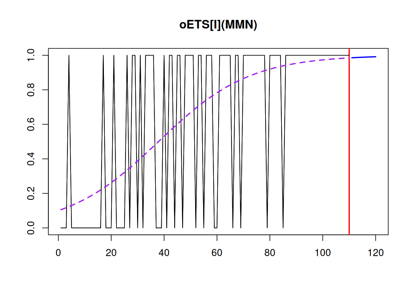
Figure 13.4: Demand occurrence and probability of occurrence in the oETS(M,M,N)\(_I\) model.
Figure 13.4 shows that similarly to the oETS\(_O\), the model captures the trend in the probability of occurrence but has a higher smoothing parameter \(\alpha_b\). Also notice how the update of states happens more often towards the second part of the data, when demand is building up and more ones appear in the data. The model is much more inert when it has many zeroes. This behaviour can be contrasted to the behaviour of oETS\(_O\), which updated the states more frequently in the beginning of the series in our example.
13.1.4 General oETS model, oETS\(_G\)
Uniting the oETS\(_O\) with oETS\(_I\), we can obtain the “general” model, which in the most general case can be summarised in the following set of state space equations: \[\begin{equation} \begin{aligned} & p_t = f_p(\mu_{a,t}, \mu_{b,t}) \\ & a_t = w_a(\mathbf{v}_{a,t-\boldsymbol{l}}) + r_a(\mathbf{v}_{a,t-\boldsymbol{l}}) \epsilon_{a,t} \\ & \mathbf{v}_{a,t} = f_a(\mathbf{v}_{a,t-\boldsymbol{l}}) + g_a(\mathbf{v}_{a,t-\boldsymbol{l}}) \epsilon_{a,t} \\ & b_t = w_b(\mathbf{v}_{b,t-\boldsymbol{l}}) + r_b(\mathbf{v}_{b,t-\boldsymbol{l}}) \epsilon_{b,t} \\ & \mathbf{v}_{b,t} = f_b(\mathbf{v}_{b,t-\boldsymbol{l}}) + g_b(\mathbf{v}_{b,t-\boldsymbol{l}}) \epsilon_{b,t} \end{aligned} , \tag{13.11} \end{equation}\] where \(\epsilon_{a,t}\), \(\epsilon_{b,t}\), \(\mu_{a,t}\), and \(\mu_{b,t}\) have been defined in previous subsections, and the other elements correspond to the ADAM discussed in Chapter 5. Note that in this case two state space models similar to the one discussed in Section 7.1 are used for the modelling of \(a_t\) and \(b_t\). These can be either ETS, or ARIMA, or regression, or any combination of those.
The general formula for the probability in the case of the multiplicative error model is: \[\begin{equation} p_t = \frac{\mu_{a,t}}{\mu_{a,t}+\mu_{b,t}} , \tag{13.12} \end{equation}\] while for the additive one, it is: \[\begin{equation} p_t = \frac{\exp(\mu_{a,t})}{\exp(\mu_{a,t})+\exp(\mu_{b,t})} . \tag{13.13} \end{equation}\] This is because both \(\mu_{a,t}\) and \(\mu_{b,t}\) need to be strictly positive, while the additive error models support negative and positive values and zero. The canonical oETS model assumes that the pure multiplicative model is used for \(a_t\) and \(b_t\). This model type is positively defined for any values of error, trend, and seasonality, which is essential for the values of \(a_t\) and \(b_t\) and their expectations. If a combination of additive and multiplicative error models is used, then the additive part should be exponentiated before using the formulae to calculate the probability. So, the \(f_p(\cdot)\) function from (13.11) maps the expectations from models A and B to the probability of occurrence, depending on the error type of the respective models:
\[\begin{equation} p_t = f_p(\mu_{a,t}, \mu_{b,t}) = \left \lbrace \begin{aligned} & \frac{\mu_{a,t}}{\mu_{a,t} + \mu_{b,t}} \text{ when both have multiplicative errors} \\ & \frac{\mu_{a,t}}{\mu_{a,t} + \exp(\mu_{b,t})} \text{ when model B has additive error} \\ & \frac{\exp(\mu_{a,t})}{\exp(\mu_{a,t}) + \mu_{b,t}} \text{ when model A has additive error} \\ & \frac{\exp(\mu_{a,t})}{\exp(\mu_{a,t}) + \exp(\mu_{b,t})} \text{ when both have additive errors.} \end{aligned} \right. \tag{13.14}\end{equation}\]
An example of the oETS model is the one based on two local level models (see discussion in Subsection 4.3), oETS\(_G\)(M,N,N)(M,N,N): \[\begin{equation} \begin{aligned} & o_t \sim \text{Bernoulli} \left(p_t \right) \\ & p_t = \frac{\mu_{a,t}}{\mu_{a,t}+\mu_{b,t}} \\ \\ & a_t = l_{a,t-1} \left(1 + \epsilon_{a,t} \right) \\ & l_{a,t} = l_{a,t-1}( 1 + \alpha_{a} \epsilon_{a,t}) \\ & \mu_{a,t} = l_{a,t-1} \\ \\ & b_t = l_{b,t-1} \left(1 + \epsilon_{b,t} \right) \\ & l_{b,t} = l_{b,t-1}( 1 + \alpha_{b} \epsilon_{b,t}) \\ & \mu_{b,t} = l_{b,t-1} \\ \end{aligned}, \tag{13.15} \end{equation}\] where all the parameters have already been defined in Subsections 13.1.2 and 13.1.3. More advanced models can be constructed for \(a_t\) and \(b_t\) by specifying the ETS models for each part and/or adding explanatory variables.
The construction of the model (13.15) is done via the following set of recursive equations: \[\begin{equation} \begin{aligned} & e_{a,t} = \frac{u_t}{1-u_t} -1 \\ & \hat{a}_t = \hat{l}_{a,t-1} \\ & \hat{l}_{a,t} = \hat{l}_{a,t-1}( 1 + \alpha_{a} e_{a,t}) \\ & e_{b,t} = \frac{1-u_t}{u_t} -1 \\ & \hat{b}_t = \hat{l}_{b,t-1} \\ & \hat{l}_{b,t} = \hat{l}_{b,t-1}( 1 + \alpha_{b} e_{b,t}) \end{aligned} . \tag{13.16} \end{equation}\]
In R, there is a separate function for the oETS\(_G\) model, called oesg(). It has twice as many parameters as oes(), because it allows fine tuning of the models for the both parts \(a_t\) and \(b_t\). This gives an additional flexibility. For example, here is how we can use ETS(M,N,N) for the \(a_t\) and ETS(A,A,N) for the \(b_t\), resulting in oETS\(_G\)(M,N,N)(A,A,N):
## Occurrence state space model estimated: General
## Underlying ETS model: oETS[G](MNN)(AAN)
##
## Sample size: 110
## Number of estimated parameters: 6
## Number of degrees of freedom: 104
## Information criteria:
##      AIC     AICc      BIC     BICc
## 106.7048 107.5203 122.9076 124.8243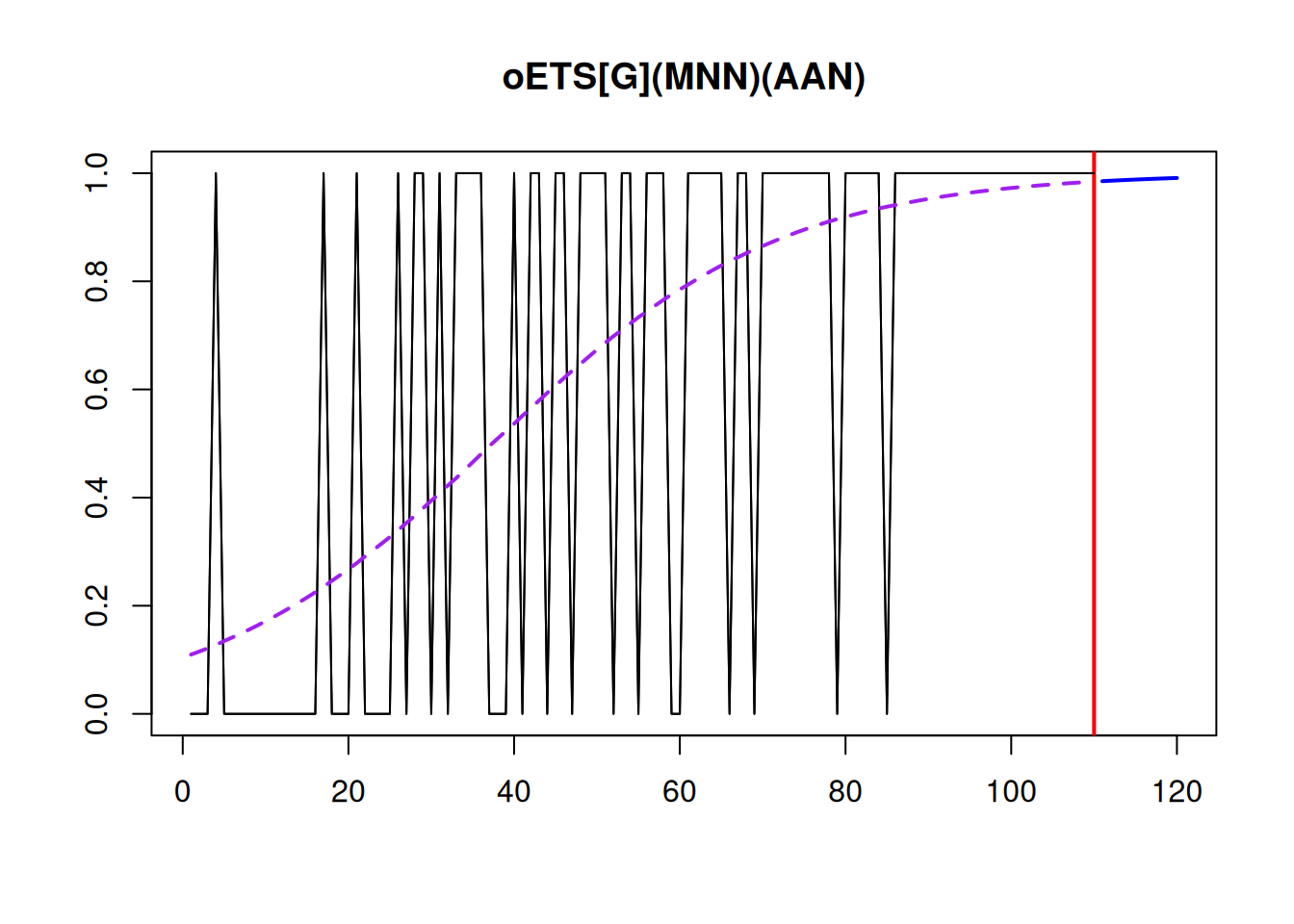
Figure 13.5: Demand occurrence and probability of occurrence in the oETS(M,N,N)(A,A,N)\(_G\) model.
We can also analyse models separately for \(a_t\) and \(b_t\) from the saved variable. Here is, for example, Model A:
## Occurrence state space model estimated: Odds ratio
## Underlying ETS model: oETS[G](MNN)_A
## Smoothing parameters:
## level
## 2e-04
## Vector of initials:
##  level
## 0.2603
##
## Error standard deviation: 1.8037
## Sample size: 110
## Number of estimated parameters: 2
## Number of degrees of freedom: 108
## Information criteria:
##      AIC     AICc      BIC     BICc
##  98.7048  98.8169 104.1057 104.3693
The experiments that I have done so far show that oETS\(_G\) very seldom brings improvements in comparison with oETS\(_O\) or oETS\(_I\) in terms of forecasting accuracy. Besides, selecting models for each of the parts is a challenging task. So, this model is theoretically attractive, being more general than the other oETS models, but is not very practical. Still it is useful because we can introduce different oETS models by restricting \(a_t\) and \(b_t\). For example, we can get:
- oETS\(_F\), when \(\mu_{a,t} = \text{const}\), \(\mu_{b,t} = \text{const}\) for all \(t\);
- oETS\(_O\), when \(\mu_{b,t} = 1\) for all \(t\);
- oETS\(_I\), when \(\mu_{a,t} = 1\) for all \(t\);
- oETS\(_D\), when \(\mu_{a,t} + \mu_{b,t} = 1\), \(\mu_{a,t} \in [0,1]\) for all \(t\) (discussed in Subsection 13.1.5);
- oETS\(_G\), when there are no restrictions.
13.1.5 Direct probability model, oETS\(_D\)
The last model in the family of oETS is the “Direct probability”. It appears, when the following restriction is imposed on the oETS\(_G\): \[\begin{equation} \mu_{a,t} + \mu_{b,t} = 1, \mu_{a,t} \in [0, 1] . \tag{13.17} \end{equation}\] This restriction is inspired by the mechanism for the probability update proposed by Teunter et al. (2011) (TSB method). Their paper uses SES (discussed in Section 3.4) to model the time-varying probability of occurrence. Based on this idea and the restriction (13.17), we can formulate an oETS\(_D\)(M,N,N) model, which will underly the occurrence part of the TSB method: \[\begin{equation} \begin{aligned} & o_t \sim \text{Bernoulli} \left(\mu_{a,t} \right) \\ & a_t = l_{a,t-1} \left(1 + \epsilon_{a,t} \right) \\ & l_{a,t} = l_{a,t-1}( 1 + \alpha_{a} \epsilon_{a,t}) \\ & \mu_{a,t} = \min(l_{a,t-1}, 1) \end{aligned}. \tag{13.18} \end{equation}\] There is also an option with the additive error for the occurrence part (also underlying TSB), which has a different, more complicated form: \[\begin{equation} \begin{aligned} & o_t \sim \text{Bernoulli} \left(\mu_{a,t} \right) \\ & a_t = l_{a,t-1} + \epsilon_{a,t} \\ & l_{a,t} = l_{a,t-1} + \alpha_{a} \epsilon_{a,t} \\ & \mu_{a,t} = \max \left( \min(l_{a,t-1}, 1), 0 \right) \end{aligned}. \tag{13.19} \end{equation}\]
The estimation of the oETS\(_D\)(M,N,M) model can be done using the following set of equations: \[\begin{equation} \begin{aligned} & \hat{\mu}_{a,t} = \hat{l}_{a,t-1} \\ & \hat{l}_{a,t} = \hat{l}_{a,t-1}( 1 + \hat{\alpha}_{a} e_{a,t}) \end{aligned}, \tag{13.20} \end{equation}\] where \[\begin{equation} e_{a,t} = \frac{o_t (1 -2 \kappa) + \kappa -\hat{\mu}_{a,t}}{\hat{\mu}_{a,t}}, \tag{13.21} \end{equation}\] and \(\kappa\) is a very small number (for example, \(\kappa = 10^{-10}\)), needed only in order to make the model estimable. The estimate of the error term in case of the additive model is much simpler and does not need any specific tricks to work: \[\begin{equation} e_{a,t} = o_t -\hat{\mu}_{a,t} , \tag{13.22} \end{equation}\] which is directly related to the TSB method. Note that equation (13.20) does not contain the minimum function, because the estimated error (13.21) will always guarantee that the level will lie between 0 and 1 as long as the smoothing parameter lies in the [0, 1] region (which is the conventional assumption for both th ETS(A,N,N) and ETS(M,N,N) models). This also applies for the oETS\(_D\)(A,N,N) model, where the maximum and minimum functions can be dropped as long as the smoothing parameter lies in [0,1].
An important feature of this model is that it allows probability to become either 0 or 1, thus implying either that there is no demand on the product or that the demand for the product has become regular. No other oETS model permits that – they assume that probability might become very close to bounds but can never reach them.
Here’s an example of the application of the oETS\(_D\)(M,M,N) to the same artificial data:
## Occurrence state space model estimated: Direct probability
## Underlying ETS model: oETS[D](MMN)
## Smoothing parameters:
## level trend
## 3e-03 6e-04
## Vector of initials:
##  level  trend
## 0.3379 1.0194
##
## Error standard deviation: 0.7594
## Sample size: 110
## Number of estimated parameters: 4
## Number of degrees of freedom: 106
## Information criteria:
##      AIC     AICc      BIC     BICc
## 109.0528 109.4338 119.8547 120.7501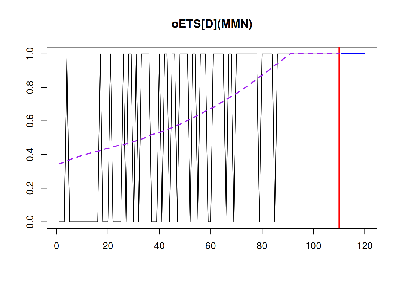
Figure 13.6: Demand occurrence and probability of occurrence in the oETS(M,M,N)\(_D\) model.
From Figure 13.6, we can see that the probability of occurrence increases rapidly and reaches the bound of one around the 90th observation.
Practically speaking, using oETS\(_D\) makes sense, when you expect the demand on your product either to disappear completely or to become regular. In other cases, oETS\(_I\) and oETS\(_O\) could be used efficiently. On M5 data, I found the latter two models to performed very well in the majority of cases (Svetunkov and Boylan, 2023a).
13.1.6 Model selection in oETS
Before we move to the model selection in oETS, it might make sense to see what sort of probability occurrence the models above are suitable for. These are summarised visually in Figure 13.7, where the random errors were generated in exactly the same fashion (with a fixed random seed) and \(\alpha=0.4\) to show the differences in dynamics between the processes.
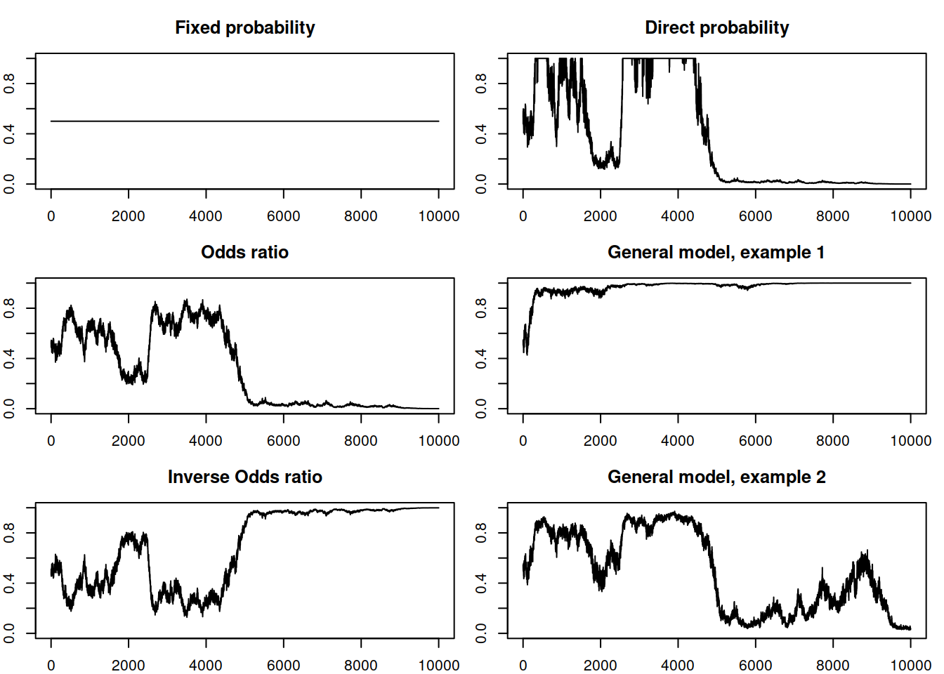
Figure 13.7: Example of several probability of occurrence processes according to oETS.
Figure 13.7 demonstrates visually what was discussed in the previous subsections related to the demand occurrence:
- The fixed probability model implies no change over time;
- The odds ratio one implies the inevitable demand obsolescence (in mathematics this corresponds to the probability almost surely converging to zero);
- The inverse odds ratio demonstrates the demand building up asymptotically (almost surely converging to one);
- The direct probability shows asymptotic behaviour similar to the oETS\(_O\), but with more rapid changes;
- And finally, the general one shows a variety of behaviours depending on the specific values of parameters for models a and b.
Hopefully, this gives a better understanding of the differences between the oETS models.
Now, when it comes to selecting the most appropriate one, there are two dimensions for the model selection in oETS:
- Selection of the type of occurrence;
- Selection of the model type for the occurrence part.
The solution in this situation is simple. Given the formula (13.4), we can try each of the models, calculate log-likelihoods, the number of all estimated parameters, and then select the one that has the lowest information criterion. The demand occurrence models discussed in this section will have:
- oETS\(_F\): 1 parameter for the probability of occurrence;
- oETS\(_O\), oETS\(_I\), and oETS\(_D\): initial values, smoothing and dampening parameters;
- oETS\(_G\): initial values, smoothing, and dampening parameters for models A and B.
For example, if the oETS(M,N,N) model is constructed, the overall number of estimated parameters for the models will be:
- oETS(M,N,N)\(_F\) – 1 parameter: the probability of occurrence \(\hat{p}\);
- oETS(M,N,N)\(_O\), oETS(M,N,N)\(_I\) and oETS(M,N,N)\(_D\) – 2 each: the initial value of level and the smoothing parameter;
- oETS(M,N,N)\(_G\) – 4: the initial values of \(\hat{l}_{a,0}\) and \(\hat{l}_{b,0}\) and the smoothing parameters \(\hat{\alpha}_a\) and \(\hat{\alpha}_b\).
This implies that the selection between models in (2) will come to the best fit to the demand occurrence data, while oETS(M,N,N)\(_G\) will only be selected if it provides a much better fit to the data. Given that intermittent demand typically does not have many observations, the selection of oETS(M,N,N)\(_G\) becomes highly improbable.
When it comes to selecting the most appropriate demand occurrence model (e.g. selecting ETS components or ARIMA orders), the approach would be similar: estimate the pool of models via likelihood, calculate numbers of parameters, select the model with the lowest information criterion. Given that we assume that the demand occurrence is independent of the demand sizes, the selection of models in the occurrence part can be done based on the likelihood (13.4) independently of the demand sizes part of the model, which significantly simplifies the estimation and model selection process for the whole iETS model.