16.1 Simulating data from ADAM
Before we move to the discussion of parameters’ uncertainty and how it propagates to the states, fitted values, and final forecasts, it makes sense to understand how data can be generated based on an ADAM with some parameters. The data generation in this case is done in the following steps:
- Decide what structure will be used for data generation. This depends on the type and order of the specific ADAM. For example, if it a pure additive ETS(A,N,A)+ARIMA(2,0,0) model then the set of equations (9.30) will be used with matrices and vectors defined by (9.31);
- Generate an error term for the values of \(t=1 \dots T\), where \(T\) is the desired sample size. The error term can be generated using any known distribution as long as its mean equals to zero in the case of additive error (\(\mathrm{E}(\epsilon_t)=0\)) or equals to one in the case of the multiplicative one (\(\mathrm{E}(1+\epsilon_t)=1\));
- Set the values of the persistence vector \(\mathbf{g}\) and the matrices \(\mathbf{w}\) and \(\mathbf{F}\). In the case of ARIMA, the values are defined based on the order of the model and the values of its parameters (see discussion in Section 9.1). The specific values will change depending on the type of model and the elements it has;
- Define the initial value of the state vector \(\mathbf{v}_t\) for \(t<1\);
- Apply recursively the formula of the state space model (7.1) (discussed in Section 7.1), collecting the values of the state vector \(\mathbf{v}_{t}\) and the generated actual values \(y_t\) for all \(t=1,\dots,T\).
Note that the simulation process allows using distributions that are not officially supported by ADAM on the step (2). In fact, in some instances the error term can be provided by a user, so it would not be random.
In the smooth package for R, there are several functions that implement this simulation procedure:
sim.es()allows generating data from an arbitrary ETS model;sim.ssarima()supports data generation from a state space ARIMA model with parameters and initial states provided by the user;sim.sma()generates data from Simple Moving Average, discussed in Subsection 3.3.3;simulate()method foradamandsmoothclasses allows generating the data using the parameters of an estimated model, thus creating time series similar to the original one.
As an example, consider estimating ADAM ETS(M,M,M) on AirPassengers data and then generating several time series from it (see Figure 16.1) using the following R code:
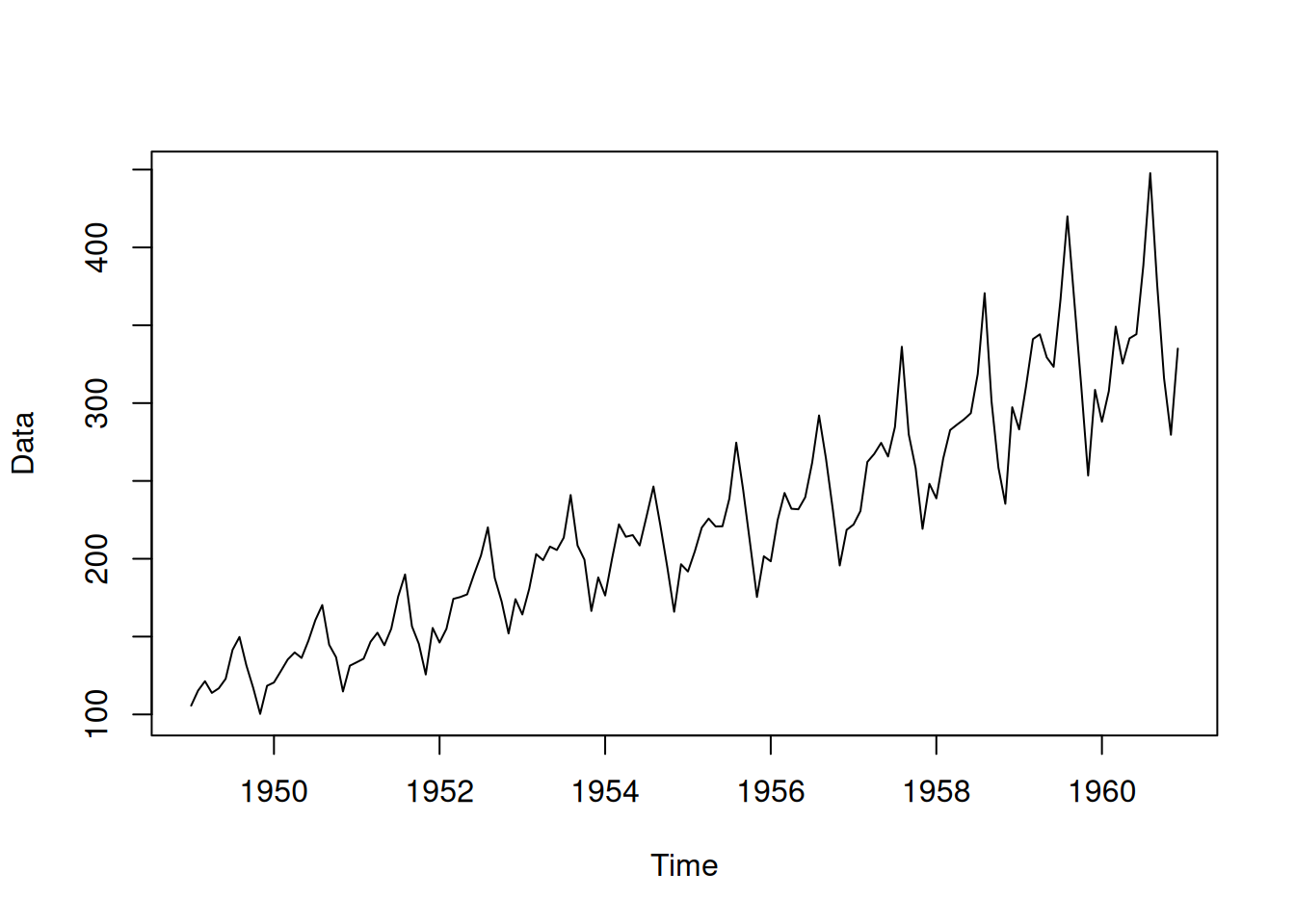
Figure 16.1: Data generated by ADAM using the parameters of the estimated ETS model.
You might notice that the trend in Figure 16.1 differs from the one in the original data. This is because the ETS model captured some changes in the trend in the data, which was then reflected in the generated series. The resulting simulated data can be used for the experiments in a controlled environment.
In some cases, some specific data might be required with specific parameters and values for the error term. In those cases, the sim.es(), sim.ssarima(), and other similar functions from the smooth package can be used. Here is an example of a code for sim.es() with an arbitrary function for the generation of the error term:
# A function to generate error term
randomizer <- function(n, mu=0, s=1){
    return(mu + s * rlogis(n, 0, 1))
}
# Generation of data from ETS(A,N,N)
x <- sim.es("ANN", obs=120, nsim=10,
            persistence=0.1, initial=1000,
            randomizer="randomizer", mu=0, s=1)
# Plot a randomly selected series from the 10 generated ones
plot(x)