10.6 Examples of application
For the example in this section, we will use the data of Road Casualties in Great Britain 1969–84, the Seatbelts dataset in the datasets package for R, which contains several variables (the description is provided in the documentation for the data and can be accessed via the ?Seatbelts command). The variable of interest, in this case is drivers, and the dataset contains more variables than needed, so we will restrict the data with drivers, kms (distance driven), PetrolPrice, and law – the latter three seem to influence the number of injured/killed drivers in principle:
The dynamics of these variables over time is shown in Figure 10.1.
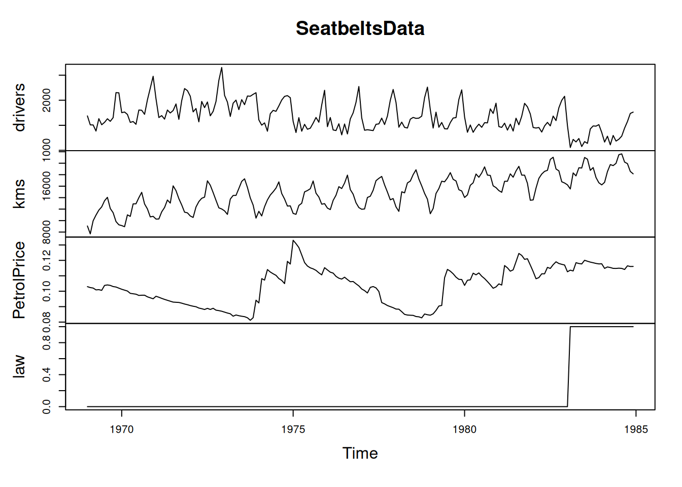
Figure 10.1: The time series dynamics of variables from Seatbelts dataset.
Apparently, the drivers variable exhibits seasonality but does not seem to have a trend. The type of seasonality is challenging to determine, but we will assume that it is multiplicative for now. A simple ETS(M,N,M) model applied to the data will produce the following (we will withhold the last 12 observations for the forecast evaluation, Figure 10.2):
adamETSMNMSeat <- adam(SeatbeltsData[,"drivers"], "MNM",
                       h=12, holdout=TRUE)
forecast(adamETSMNMSeat, h=12, interval="prediction") |>
    plot()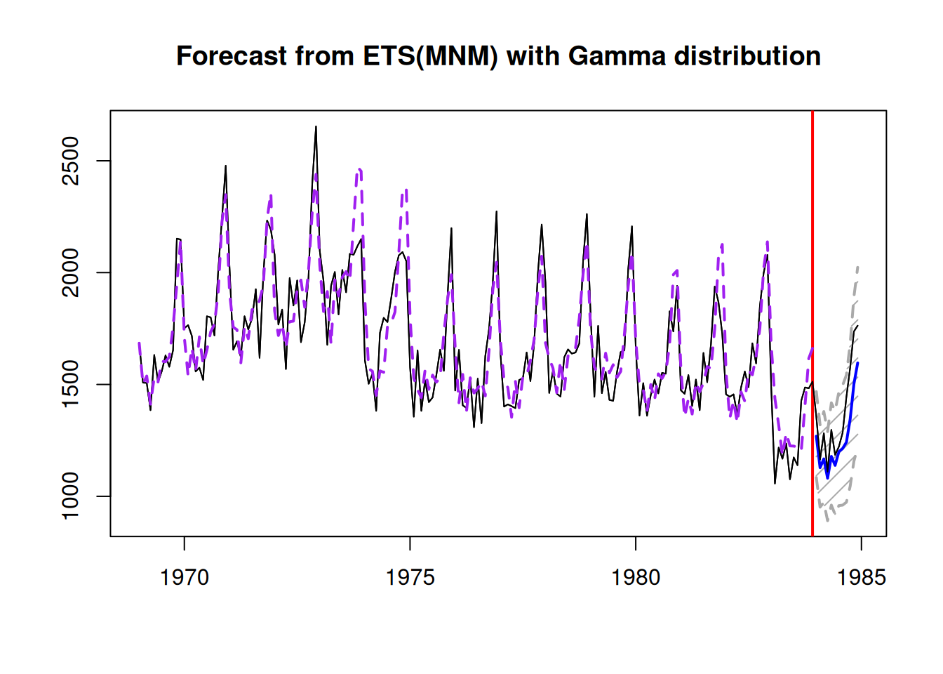
Figure 10.2: The actual values for drivers and a forecast from an ETS(M,N,M) model.
This simple model already does a fine job fitting the data and producing forecasts. However, the forecast is biased and is consistently lower than needed because of the sudden drop in the level of series, which can only be explained by the introduction of the new law in the UK in 1983, making the seatbelts compulsory for drivers. Due to the sudden drop, the smoothing parameter for the level of series is higher than needed, leading to wider intervals and less accurate forecasts. Here is the output of the model:
## Time elapsed: 0.02 seconds
## Model estimated using adam() function: ETS(MNM)
## With backcasting initialisation
## Distribution assumed in the model: Gamma
## Loss function type: likelihood; Loss function value: 1130.312
## Persistence vector g:
##  alpha  gamma
## 0.3998 0.0408
##
## Sample size: 180
## Number of estimated parameters: 3
## Number of degrees of freedom: 177
## Information criteria:
##      AIC     AICc      BIC     BICc
## 2266.624 2266.760 2276.202 2276.556
##
## Forecast errors:
## ME: 113.372; MAE: 113.372; RMSE: 135.904
## sCE: 80.48%; Asymmetry: 100%; sMAE: 6.707%; sMSE: 0.646%
## MASE: 0.657; RMSSE: 0.603; rMAE: 0.485; rRMSE: 0.535
In order to further explore the data we will produce the scatterplots and boxplots between the variables using the spread() function from the greybox package (Figure 10.3):
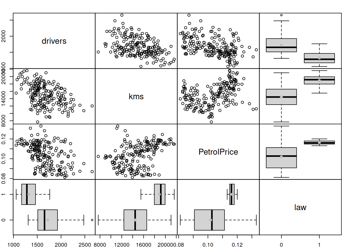
Figure 10.3: The relation between variables from the Seatbelts dataset.
Figure 10.3 shows a negative relation between kms and drivers: the higher the distance driven, the lower the total of car drivers killed or seriously injured. A similar relation is observed between the petrol price and drivers (when the prices are high, people tend to drive less, thus causing fewer incidents). Interestingly, the increase of both variables causes the variance of the response variable to decrease (heteroscedasticity effect). Using a multiplicative error model and including the variables in logarithms, in this case, might address this potential issue. Note that we do not need to take the logarithm of drivers, as we already use the model with multiplicative error. Finally, the legislation of a new law seems to have caused a decrease in the number of causalities. To have a better model in terms of explanatory and predictive power, we should include all three variables. This is how we can do that using adam():
adamETSXMNMSeat <- adam(SeatbeltsData, "MNM", h=12, holdout=TRUE,
                        formula=drivers~log(kms)+log(PetrolPrice)+law)
The parameter formula in general is not compulsory. It can either be substituted by “formula=drivers~.” or dropped completely – in the latter case, the function would fit the model of the first variable in the matrix from everything else. We need the formula in our case because we introduce log-transformations of some explanatory variables.
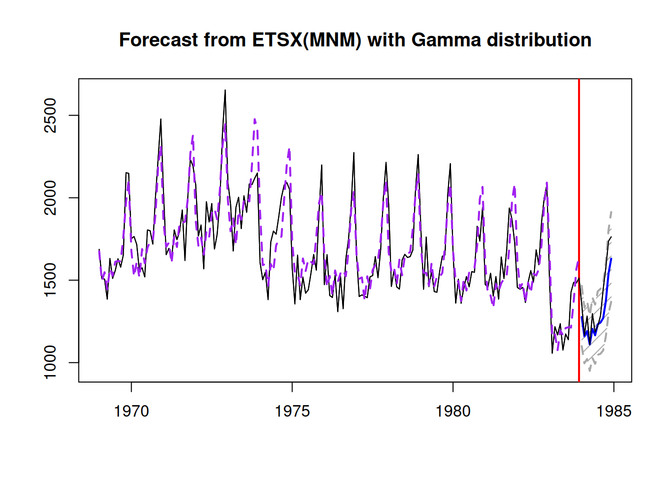
Figure 10.4: The actual values for drivers and a forecast from an ETSX(M,N,M) model.
Figure 10.4 shows the forecast from the second model, which is slightly more accurate. More importantly, the prediction interval is narrower than in the simple ETS(M,N,M) because now the model takes the external information into account. Here is the summary of the second model:
## Time elapsed: 0.09 seconds
## Model estimated using adam() function: ETSX(MNM)
## With backcasting initialisation
## Distribution assumed in the model: Gamma
## Loss function type: likelihood; Loss function value: 1117.482
## Persistence vector g (excluding xreg):
##  alpha  gamma
## 0.1780 0.0389
##
## Sample size: 180
## Number of estimated parameters: 6
## Number of degrees of freedom: 174
## Information criteria:
##      AIC     AICc      BIC     BICc
## 2246.963 2247.449 2266.121 2267.382
##
## Forecast errors:
## ME: 85.343; MAE: 87.236; RMSE: 112.854
## sCE: 60.583%; Asymmetry: 94.6%; sMAE: 5.161%; sMSE: 0.446%
## MASE: 0.506; RMSSE: 0.501; rMAE: 0.373; rRMSE: 0.444
Note that the smoothing parameter \(\alpha\) has reduced from 0.4 to 0.18. This led to the reduction in error measures. For example, based on RMSE, we can conclude that the model with explanatory variables is more precise than the simple univariate ETS(M,N,M). Still, we could try introducing the update of the parameters for the explanatory variables to see how it works (it might be unnecessary for this data):
adamETSXMNMDSeat <- adam(SeatbeltsData, "MNM", h=12, holdout=TRUE,
                         formula=drivers~log(kms)+log(PetrolPrice)+law,
regressors="adapt", maxeval=10000)Remark. Given the complexity of the estimation task, the default number of iterations needed for the optimiser to find the minimum of the loss function might not be sufficient. This is why I introduced maxeval=10000 in the code above, increasing the number of maximum iterations to 10,000. In order to see how the optimiser worked out, you can add print_level=41 in the code above.
In our specific case, the difference between the ETSX and ETSX{D} models is infinitesimal in terms of the accuracy of final forecasts and prediction intervals. Here is the output of the model:
## Time elapsed: 0.18 seconds
## Model estimated using adam() function: ETSX(MNM){D}
## With backcasting initialisation
## Distribution assumed in the model: Gamma
## Loss function type: likelihood; Loss function value: 1117.243
## Persistence vector g (excluding xreg):
##  alpha  gamma
## 0.1376 0.0390
##
## Sample size: 180
## Number of estimated parameters: 9
## Number of degrees of freedom: 171
## Information criteria:
##      AIC     AICc      BIC     BICc
## 2252.486 2253.545 2281.223 2283.972
##
## Forecast errors:
## ME: 87.186; MAE: 88.662; RMSE: 114.264
## sCE: 61.891%; Asymmetry: 96.1%; sMAE: 5.245%; sMSE: 0.457%
## MASE: 0.514; RMSSE: 0.507; rMAE: 0.379; rRMSE: 0.45
We can spot that the error measures of the dynamic model are slightly lower than the ones from the static one (e.g., compare RMSE of models). However, the AICc is slightly higher. This means that the two models are very similar in terms of their performance. So, I decided to use the dynamic model for forecasting and analytical purposes because it has lower smoothing parameters. In order to see the set of smoothing parameters for the explanatory variables in this model, we can use the command:
##  alpha  gamma delta1 delta2 delta3
## 0.1376 0.0390 0.0104 0.0319 0.0000
And see how the states/parameters of the model change over time (Figure 10.5):
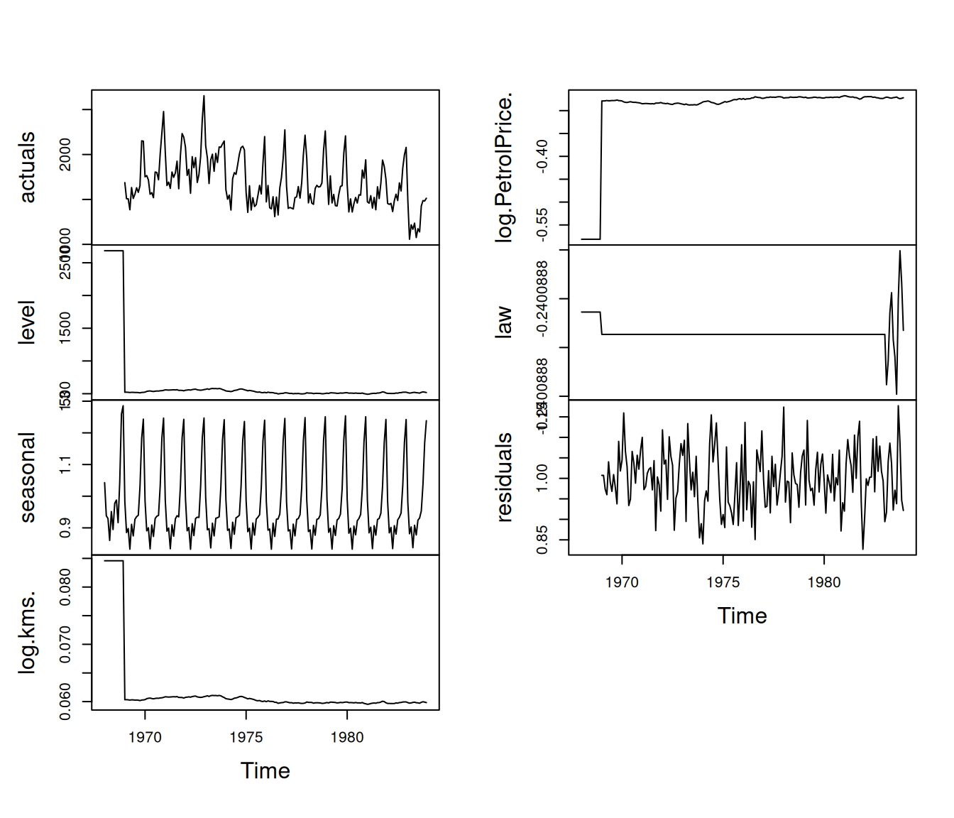
Figure 10.5: Dynamic of states of the ETSX(M,N,M){D} model.
As we see in Figure 10.5, the effects of variables change over time. This mainly applies to the PetrolPrice variable, the smoothing parameter for which is the highest among all \(\delta_i\) parameters.
To see the initial effects of the explanatory variables on the number of incidents with drivers, we can look at the parameters for those variables:
##         log.kms. log.PetrolPrice.              law
##       0.08458772      -0.58129402      -0.24008880
Based on that, we can conclude that the introduction of the law reduced on average the number of incidents by approximately 24%, while the increase of the petrol price by 1% leads on average to a decrease in the number of incidents by 0.28%. Finally, the distance negatively impacts the incidents as well, reducing it on average by 0.1% for each 1% increase in the distance. This is the standard interpretation of parameters, which we can use based on the estimated model (see, for example, discussion in Section 11.3 of Svetunkov and Yusupova, 2025). We will discuss how to do further analysis using ADAM in Chapter 16, introducing the standard errors and confidence intervals for the parameters.
Finally, adam() has some shortcuts when a matrix of variables (not a data frame!) is provided with no formula, assuming that the necessary expansion has already been done. This leads to the decrease in computational time of the function and becomes especially useful when working on large samples of data. Here is an example with ETSX(M,N,N):
# Create matrix for the model
SeatbeltsDataExpanded <-
  ts(model.frame(drivers~log(kms)+log(PetrolPrice)+law,
                 SeatbeltsData),
     start=start(SeatbeltsData), frequency=frequency(SeatbeltsData))
# Fix the names of variables
colnames(SeatbeltsDataExpanded) <-
  make.names(colnames(SeatbeltsDataExpanded))
# Apply the model
adamETSXMNMExpandedSeat <- adam(SeatbeltsDataExpanded, "MNM",
                                lags=12, h=12, holdout=TRUE)