16.3 Confidence intervals for parameters
As it is well known in statistics (e.g. see Section 6.4 of Svetunkov and Yusupova, 2025), if several vital model assumptions (discussed in Section 14) are satisfied and CLT holds, then the distribution of estimates of parameters will follow the Normal one, which will allow us to construct confidence intervals to capture the uncertainty around the parameters. In cases of ETS and ARIMA models in the ADAM framework, the estimated parameters include smoothing, dampening, and ARMA parameters together with the initial states. In the case of explanatory variables, the pool of parameters is increased by the coefficients for those variables and their smoothing parameters (if the dynamic model from Section 10.3 is used). Furthermore, in the case of the intermittent state space model, the parameters will also include the elements of the occurrence part of the model. The CLT should hold for all of them if:
- Estimates of parameters are consistent (e.g. MSE or likelihood is used in estimation, see Section 11);
- The parameters do not lie near the bounds;
- The model is correctly specified;
- Moments of the distribution of error term are finite.
In case of ETS and ARIMA, some of the parameters are bounded (e.g. to satisfy stability condition from Section 5.4), and the estimates might lie near the bounds. This means that the distribution of estimates of parameters might not be Normal. However, given that the bounds of the parameters are typically fixed, and all estimates that exceed them are set to the boundary values in the optimisation routine, the estimates of parameters will follow Rectified Normal distribution (Socci et al., 1997). This is important because knowing the distribution, we can derive the confidence intervals for the parameters. However, given that we estimate the standard errors of parameters in-sample, we need to use t-statistics to correctly capture the uncertainty. The confidence intervals will be constructed in a conventional way in this case, using the formula (see Section 6.4 of Svetunkov and Yusupova, 2025): \[\begin{equation} \theta_j \in (\hat{\theta_j} + t_{\alpha/2}(df) s_{\theta_j}, \hat{\theta_j} + t_{1-\alpha/2}(df) s_{\theta_j}), \tag{16.2} \end{equation}\] where \(t_{\alpha/2}(df)\) is Student’s t-statistics for \(df=T-k\) degrees of freedom (\(T\) is the sample size and \(k\) is the number of all estimated parameters) and \(\alpha\) is the significance level. Then, after constructing the intervals, we can cut their values with the bounds of parameters, thus rectifying the distribution.
To construct the interval, we need to know the standard errors of parameters. Luckily, they can be calculated as square roots of the diagonal of the covariance matrix of parameters (discussed in Section 16.2):
##      alpha       beta        phi
## 0.10925210 0.10927024 0.07209241
Based on these values and the formula (16.2), we can produce confidence intervals for the parameters of any ADAM, which is done in R using the confint() method. For example, here are the intervals for the model estimated before with the significance level of 1% (confidence level of 99%):
##             S.E.       0.5%     99.5%
## alpha 0.10925210 0.65455077 1.0000000
## beta  0.10927024 0.01429301 0.5849967
## phi   0.07209241 0.68965843 1.0000000
In the output above, the distributions for \(\alpha\), \(\beta\), and \(\phi\) are rectified: \(\alpha\) and \(\phi\) are restricted with the region (0, 1) and thus are rectified from above, while \(\beta \in (0, \alpha)\) and as a result is rectified from below.
Remark. We do not rectify the distribution of \(\beta\) from above, because \(\hat{\alpha} \approx\) 0.94.
To have the bigger picture, we can produce the summary of the model, which will include the table above:
##
## Model estimated using adam() function: ETS(AAdN)
## Response variable: BJsales
## Distribution used in the estimation: Normal
## Loss function type: likelihood; Loss function value: 240.2383
## Coefficients:
##       Estimate Std. Error Lower 0.5% Upper 99.5%
## alpha   0.9400     0.1093     0.6546       1.000 *
## beta    0.2998     0.1093     0.0143       0.585 *
## phi     0.8780     0.0721     0.6897       1.000 *
##
## Error standard deviation: 1.3655
## Sample size: 140
## Number of estimated parameters: 4
## Number of degrees of freedom: 136
## Information criteria:
##      AIC     AICc      BIC     BICc
## 488.4765 488.7728 500.2431 500.9752
The output above shows the estimates of parameters and their 99% confidence intervals. Based on this output, for example, we can conclude that the uncertainty about the initial trend estimate is large, and in the “true model”, it could be either positive or negative (or even close to zero). At the same time, the “true” parameter of the initial level will lie in 99% of the cases between 190.4172 and 215.0740. Just as a reminder, Figure 16.2 shows the model fit and point forecasts for the estimated ETS model on this data.
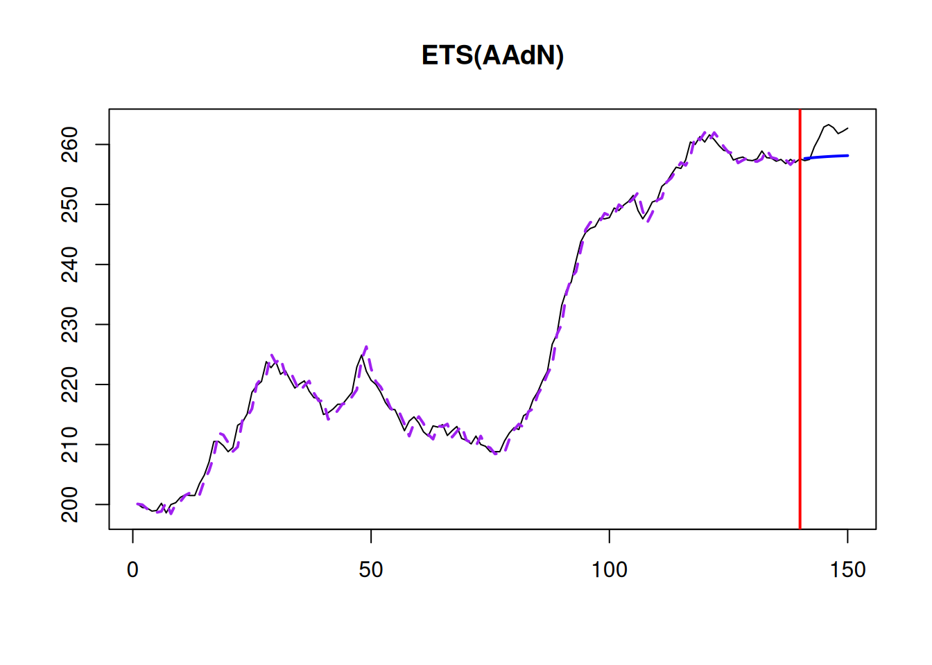
Figure 16.2: Model fit and point forecasts of ETS(A,Ad,N) on Box-Jenkins sales data.
As another example, we can have a similar summary for ARIMA models in ADAM:
##
## Model estimated using auto.adam() function: ARIMA(2,1,2) with drift
## Response variable: BJsales
## Distribution used in the estimation: Normal
## Loss function type: likelihood; Loss function value: 239.7032
## Coefficients:
##           Estimate Std. Error Lower 2.5% Upper 97.5%
## phi1[1]    -0.0896     0.1248    -0.3364      0.1569
## phi2[1]     0.7644     0.1141     0.5388      0.9899 *
## theta1[1]   0.2727     0.1627    -0.0491      0.5943
## theta2[1]  -0.5125     0.1462    -0.8017     -0.2236 *
## drift       0.1424     0.1163    -0.0875      0.3722
##
## Error standard deviation: 1.3704
## Sample size: 140
## Number of estimated parameters: 6
## Number of degrees of freedom: 134
## Information criteria:
##      AIC     AICc      BIC     BICc
## 491.4065 492.0381 509.0563 510.6169
From the summary above, we can see that the parameter \(\phi_2\) is close to zero, and the interval around it is wide. So, we can expect that it might change the sign if the sample size increases or become even closer to zero. Given that the model above was estimated with the optimisation of initial states, we also see the values for the ARIMA states and their confidence intervals in the summary above. If we used initial="backcasting", the summary would not include them.
Remark. If we faced difficulties estimating the covariance matrix of parameters using the standard Hessian-based approach, we could try bootstrap via summary(adamETSBJ, bootstrap=TRUE).
This estimate of uncertainty via confidence intervals might also be helpful to see what can happen with the estimates of parameters if the sample size increases: will they change substantially or not? If they do, then the decisions made on Monday based on the available data might differ considerably from the decisions made on Tuesday. So, in the ideal world, we would want to have as narrow confidence intervals of parameters as possible.