3.4 Simple Exponential Smoothing
One of the most powerful and efficient forecasting methods for level time series (which is also very popular in practice according to Weller and Crone, 2012) is Simple Exponential Smoothing (sometimes also called “Single Exponential Smoothing”). It was first formulated by Brown (1956) and can be written as: \[\begin{equation} \hat{y}_{t+1} = \hat{\alpha} {y}_{t} + (1 -\hat{\alpha}) \hat{y}_{t}, \tag{3.17} \end{equation}\] where \(\hat{\alpha}\) is the smoothing parameter, which is typically restricted within the (0, 1) region (this region is arbitrary, and we will see in Section 4.7 what is the correct one). This is one of the simplest forecasting methods. The smoothing parameter is typically interpreted as a weight between the latest actual value and the one-step-ahead predicted one. If the smoothing parameter is close to zero, then more weight is given to the previous fitted value \(\hat{y}_{t}\) and the new information is neglected. If \(\hat{\alpha}=0\), then the method becomes equivalent to the Global Mean method, discussed in Subsection 3.3.2. When it is close to one, then most of the weight is assigned to the actual value \({y}_{t}\). If \(\hat{\alpha}=1\), then the method transforms into Naïve, discussed in Subsection 3.3.1. By changing the smoothing parameter value, the forecaster can decide how to approximate the data and filter out the noise.
Also, notice that this is a recursive method, meaning that there needs to be some starting point \(\hat{y}_1\) to apply (3.17) to the existing data. Different initialisation and estimation methods for SES have been discussed in the literature. Still, the state of the art one is to estimate \(\hat{\alpha}\) and \(\hat{y}_{1}\) together by minimising some loss function (Hyndman et al., 2002). Typically MSE (see Section 2.1) is used, minimising the squares of one step ahead in-sample forecast error.
3.4.1 Examples of application
Here is an example of how this method works on different time series. We start with generating a stationary series and using the es() function from the smooth package. Although it implements the ETS model, we will see in Section 4.3 the connection between SES and ETS(A,N,N). We start with the stationary time series and \(\hat{\alpha}=0\):
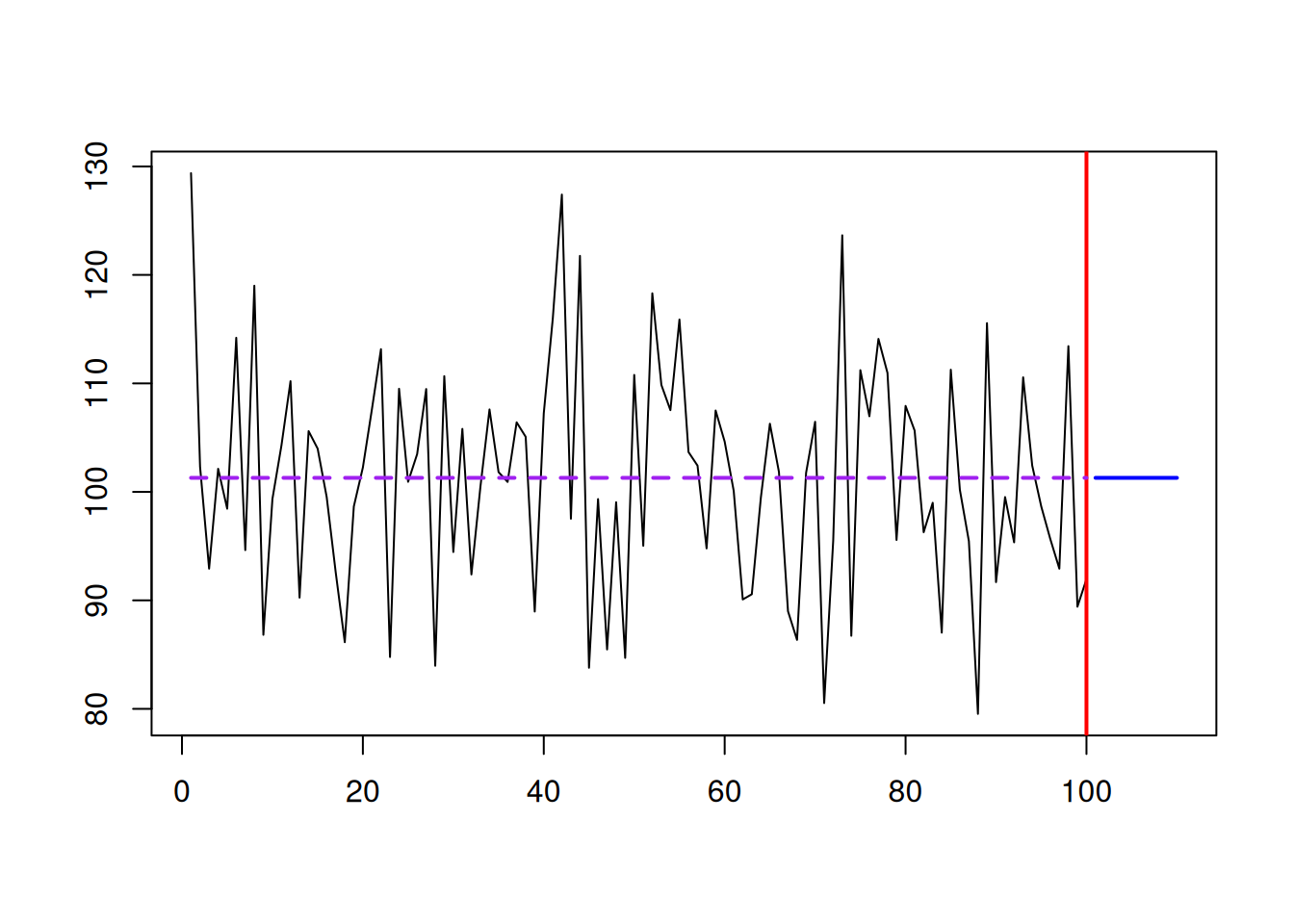
Figure 3.14: An example with a time series and SES forecast. \(\hat{\alpha}=0.\)
As we see from Figure 3.14, the SES works well in this case, capturing the deterministic level of the series and filtering out the noise. In this case, it works like a global average applied to the data. As mentioned before, the method is flexible, so if we have a level shift in the data and increase the smoothing parameter, it will adapt and get to the new level. Figure 3.15 shows an example with a level shift in the data.
y <- c(rnorm(50,100,10),rnorm(50,130,10))
es(y, model="ANN", h=10, persistence=0.1) |>
    plot(7, main="")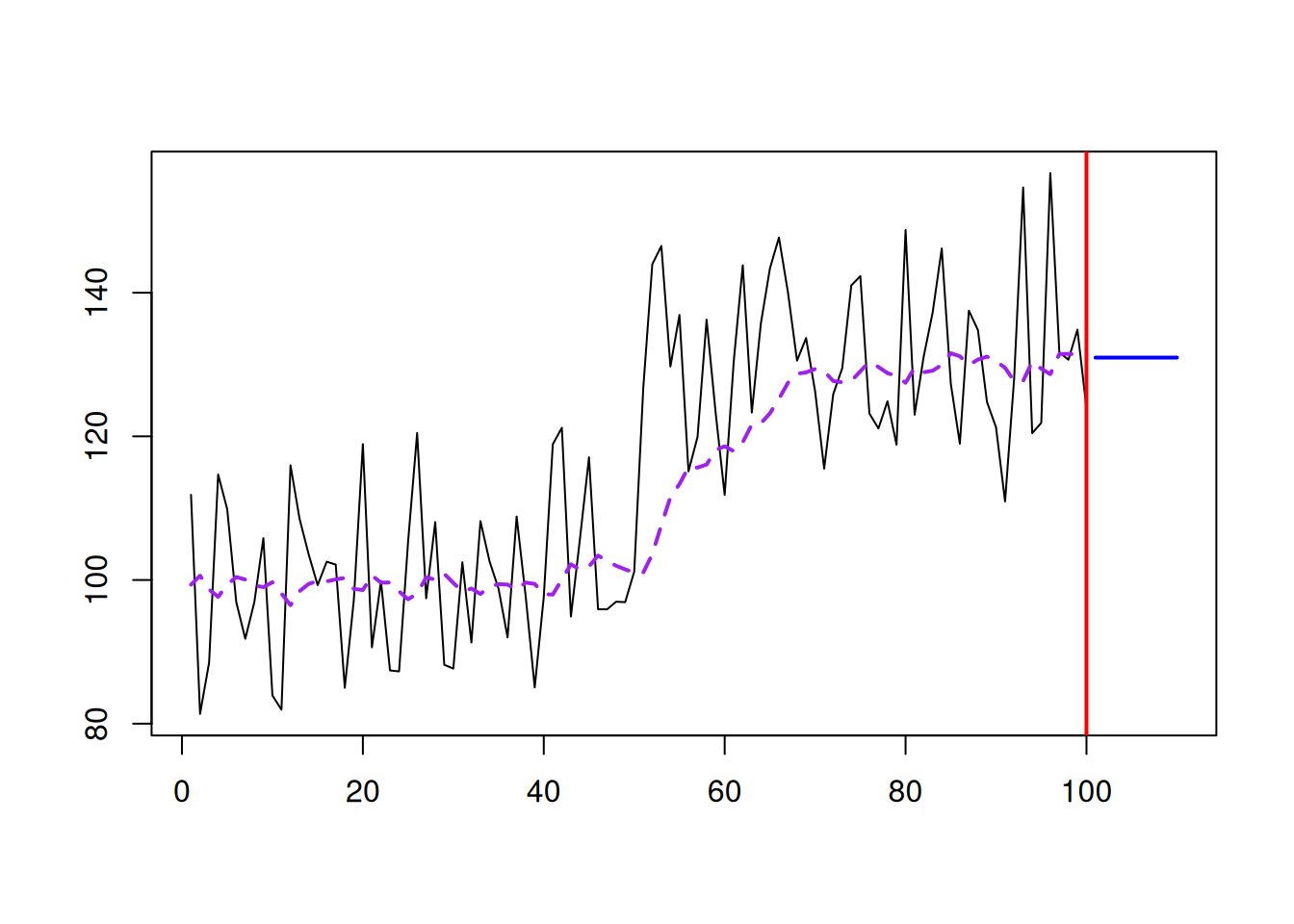
Figure 3.15: An example with a time series and SES forecast. \(\hat{\alpha}=0.1.\)
With \(\hat{\alpha}=0.1\), SES manages to get to the new level, but now the method starts adapting to noise a little bit – it follows the peaks and troughs and repeats them with a lag, but with a much smaller magnitude (see Figure 3.15). Increasing the smoothing parameter, the model will react to the changes much faster, at the cost of responding more to noise. This is shown in Figure 3.16 with different smoothing parameter values.
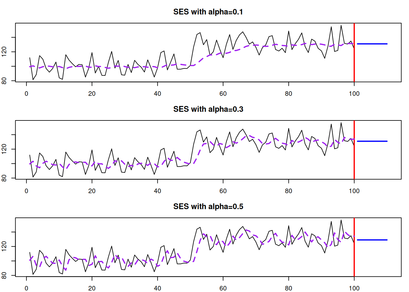
Figure 3.16: SES with different smoothing parameters applied to the same data.
If we set \(\hat{\alpha}=1\), we will end up with the Naïve forecasting method (see Section 3.3.1), which is not appropriate for our example (see Figure 3.17).
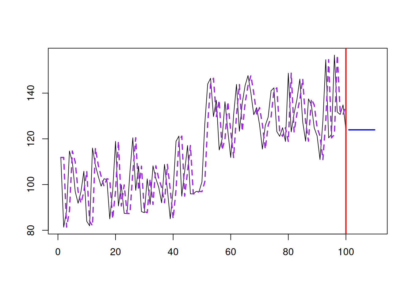
Figure 3.17: SES with \(\hat{\alpha}=1\).
So, when working with SES, we need to make sure that the reasonable smoothing parameter is selected. This can be done automatically via minimising the in-sample MSE (see Figure 3.18):
ourModel <- es(y, model="ANN", h=10, loss="MSE")
plot(ourModel, 7, main=paste0("SES with alpha=",
                              round(ourModel$persistence,3)))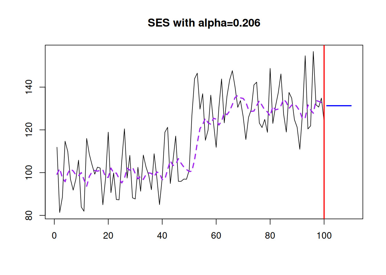
Figure 3.18: SES with optimal smoothing parameter.
This approach won’t guarantee that we will get the most appropriate \(\hat{\alpha}\). Still, it has been shown in the literature that the optimisation of smoothing parameters on average leads to improvements in terms of forecasting accuracy (see, for example, Gardner, 1985).
3.4.2 Why “exponential”?
Now, why is it called “exponential”? Because the same method can be represented in a different form, if we substitute \(\hat{y}_{t}\) in right-hand side of (3.17): \[\begin{equation*} \hat{y}_{t+1} = \hat{\alpha} {y}_{t} + (1 -\hat{\alpha}) \hat{y}_{t}, \end{equation*}\] by the same formula for the previous step (i.e. shifting all time indices by one): \[\begin{equation*} \hat{y}_{t} = \hat{\alpha} {y}_{t-1} + (1 -\hat{\alpha}) \hat{y}_{t-1}, \end{equation*}\] we will get: \[\begin{equation} \begin{aligned} \hat{y}_{t+1} = &\hat{\alpha} {y}_{t} + (1 -\hat{\alpha}) \hat{y}_{t} = \\ & \hat{\alpha} {y}_{t} + (1 -\hat{\alpha}) \left( \hat{\alpha} {y}_{t-1} + (1 -\hat{\alpha}) \hat{y}_{t-1} \right). \end{aligned} \tag{3.18} \end{equation}\] By repeating this procedure for each \(\hat{y}_{t-1}\), \(\hat{y}_{t-2}\), etc., we will obtain a different form of the method: \[\begin{equation} \hat{y}_{t+1} = \hat{\alpha} {y}_{t} + \hat{\alpha} (1 -\hat{\alpha}) {y}_{t-1} + \hat{\alpha} (1 -\hat{\alpha})^2 {y}_{t-2} + \dots + \hat{\alpha} (1 -\hat{\alpha})^{t-1} {y}_{1} + (1 -\hat{\alpha})^t \hat{y}_1 \tag{3.19} \end{equation}\] or equivalently: \[\begin{equation} \hat{y}_{t+1} = \hat{\alpha} \sum_{j=0}^{t-1} (1 -\hat{\alpha})^j {y}_{t-j} + (1 -\hat{\alpha})^t \hat{y}_1 . \tag{3.20} \end{equation}\] In the form (3.20), each actual observation has a weight in front of it. For the most recent observation, it is equal to \(\hat{\alpha}\), for the previous one, it is \(\hat{\alpha} (1 -\hat{\alpha})\), then \(\hat{\alpha} (1 -\hat{\alpha})^2\), etc. These form the geometric series or an exponential curve. Figure 3.19 shows an example with \(\hat{\alpha} =0.25\) for a sample of 30 observations.
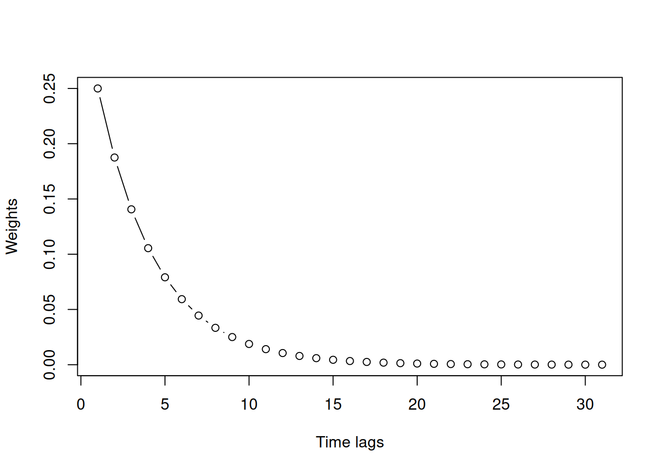
Figure 3.19: Example of weights distribution for \(\hat{\alpha}=0.25.\)
This explains the name “exponential”. The term “smoothing” comes from the idea that the parameter \(\hat{\alpha}\) should be selected so that the method smooths the original time series and does not react to noise.
3.4.3 Error correction form of SES
Finally, there is an alternative form of SES, known as error correction form, which can be obtained after some simple permutations. Taking that \(e_t=y_t-\hat{y}_t\) is the one step ahead forecast error, formula (3.17) can be written as: \[\begin{equation} \hat{y}_{t+1} = \hat{y}_{t} + \hat{\alpha} e_{t}. \tag{3.21} \end{equation}\] In this form, the smoothing parameter \(\hat{\alpha}\) has a different meaning: it regulates how much the model reacts to the previous forecast error. In this interpretation, it no longer needs to be restricted with (0, 1) region, but we would still typically want it to be closer to zero to filter out the noise, not to adapt to it.
As you see, SES is a straightforward method. It is easy to explain to practitioners, and it is very easy to implement in practice. However, this is just a forecasting method (see Section 1.4), so it provides a way of generating point forecasts but does not explain where the error comes from and how to create prediction intervals. Over the years, this was a serious limitation of the method until the introduction of state space models and ETS.