6.7 Examples of application
6.7.1 Non-seasonal data
We continue our examples with the same Box-Jenkins sales data by fitting the ETS(M,M,N) model, but this time with a holdout of ten observations:
## Time elapsed: 0.04 seconds
## Model estimated using adam() function: ETS(MMN)
## With backcasting initialisation
## Distribution assumed in the model: Gamma
## Loss function type: likelihood; Loss function value: 245.3758
## Persistence vector g:
##  alpha   beta
## 1.0000 0.2406
##
## Sample size: 140
## Number of estimated parameters: 5
## Number of degrees of freedom: 135
## Information criteria:
##      AIC     AICc      BIC     BICc
## 500.7515 501.1993 515.4597 516.5661
##
## Forecast errors:
## ME: 3.219; MAE: 3.331; RMSE: 3.786
## sCE: 14.132%; Asymmetry: 91.6%; sMAE: 1.463%; sMSE: 0.028%
## MASE: 2.818; RMSSE: 2.483; rMAE: 0.925; rRMSE: 0.922
The output above is similar to the one we discussed in Section 5.6, so we can compare the two models using various criteria and select the most appropriate. Even though the default distribution for the multiplicative error models in ADAM is Gamma, we can compare this model with the ETS(A,A,N) via information criteria. For example, here are the AICc for the two models:
## [1] 501.1993## [1] 497.0242The comparison is fair because both models were estimated via likelihood, and both likelihoods are formulated correctly, without omitting any terms (e.g. the ets() function from the forecast package omits the \(-\frac{T}{2} \log\left(2\pi e \frac{1}{T}\right)\) for convenience, which makes it incomparable with other models). In this example, the pure additive model is more suitable for the data than the pure multiplicative one.
Figure 6.2 shows how the model fits the data and what forecast it produces. Note that the function produces the point forecast in this case, which is not equivalent to the conditional expectation! The point forecast undershoots the actual values in the holdout.
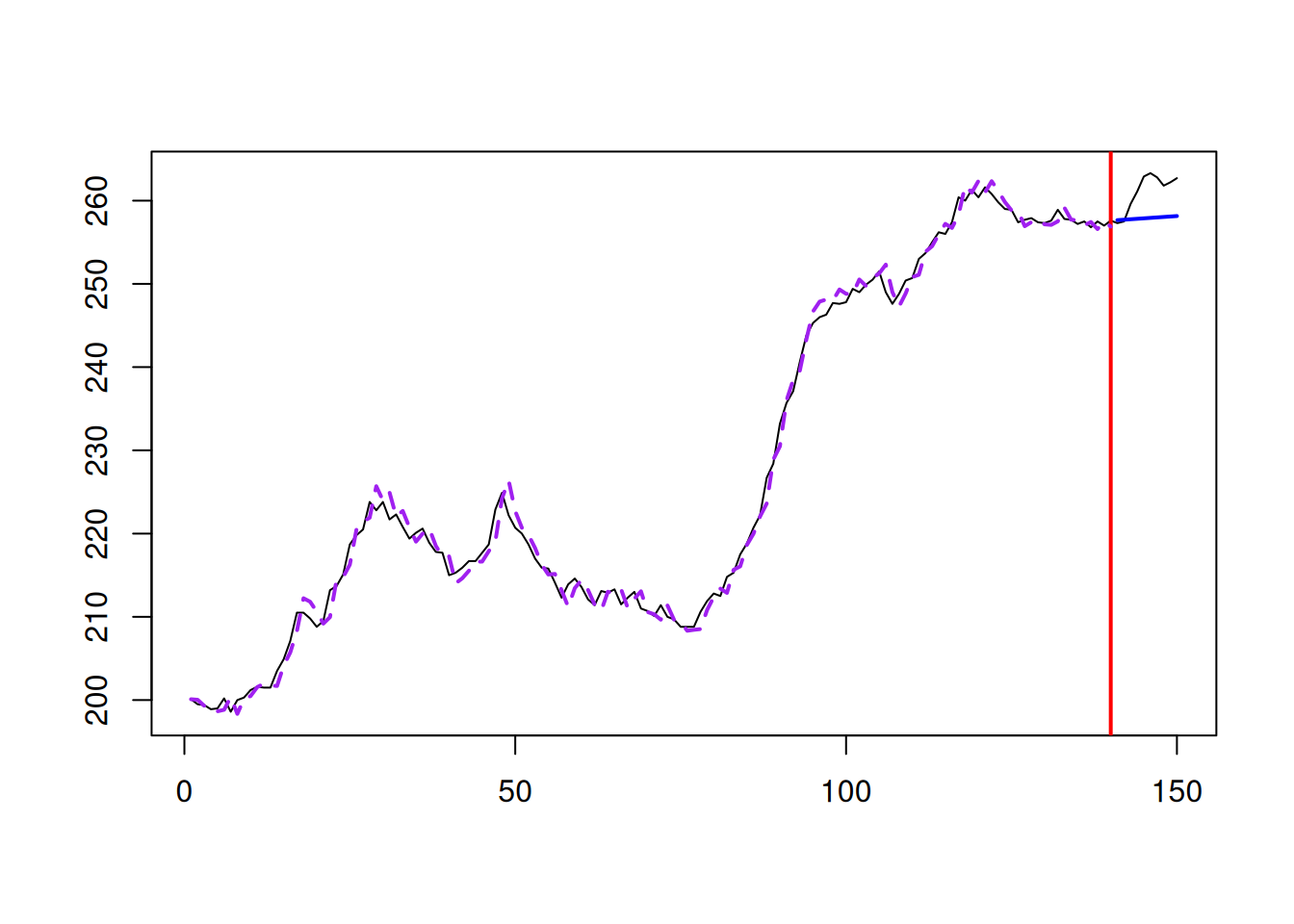
Figure 6.2: Model fit for Box-Jenkins sales data from ETS(M,M,N).
If we want to produce the forecasts (conditional expectation and prediction interval) from the model, we can do it, using the same command as in Section 5.6:
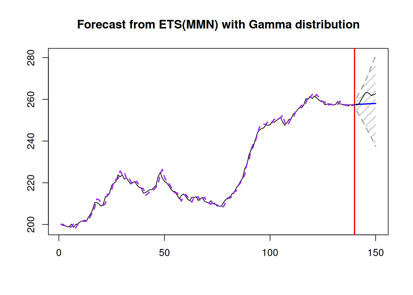
Figure 6.3: Forecast for Box-Jenkins sales data from ETS(M,M,N).
Note that, when we ask for “prediction” interval, the forecast() function will automatically decide what to use based on the estimated model: in the case of a pure additive one, it will use analytical solutions, while in the other cases, it will use simulations (see Section 18.3). The point forecast obtained from the forecast function corresponds to the conditional expectation and is calculated based on the simulations. This also means that it will differ slightly from one run of the function to another (reflecting the uncertainty in the error term). Still, the difference, in general, should be negligible for a large number of simulation paths.
The forecast with prediction interval is shown in Figure 6.3. The conditional expectation is not very different from the point forecast in this example. This is because the variance of the error term is close to zero, thus bringing the two close to each other:
## [1] 3.899779e-05We can also compare the performance of ETS(M,M,N) with Gamma distribution with the conventional ETS(M,M,N) assuming normality:
## Time elapsed: 0.04 seconds
## Model estimated using adam() function: ETS(MMN)
## With backcasting initialisation
## Distribution assumed in the model: Normal
## Loss function type: likelihood; Loss function value: 245.3869
## Persistence vector g:
##  alpha   beta
## 1.0000 0.2422
##
## Sample size: 140
## Number of estimated parameters: 5
## Number of degrees of freedom: 135
## Information criteria:
##      AIC     AICc      BIC     BICc
## 500.7738 501.2216 515.4820 516.5884
##
## Forecast errors:
## ME: 3.213; MAE: 3.327; RMSE: 3.78
## sCE: 14.108%; Asymmetry: 91.6%; sMAE: 1.461%; sMSE: 0.028%
## MASE: 2.814; RMSSE: 2.48; rMAE: 0.924; rRMSE: 0.92
In this specific example, the two distributions produce very similar results with almost indistinguishable estimates of parameters.
6.7.2 Seasonal data
The AirPassengers data used in Section 5.6 has (as we discussed) multiplicative seasonality. So, the ETS(M,M,M) model might be more suitable than the pure additive one that we used previously:
After running the command above we might get a warning, saying that the model has a potentially explosive multiplicative trend. This happens, when the final in-sample value of the trend component is greater than one, in which case the forecast trajectory might exhibit exponential growth. Here is what we have in the output of this model:
## Time elapsed: 0.16 seconds
## Model estimated using adam() function: ETS(MMM)
## With backcasting initialisation
## Distribution assumed in the model: Gamma
## Loss function type: likelihood; Loss function value: 474.0411
## Persistence vector g:
##  alpha   beta  gamma
## 0.4517 0.0005 0.4129
##
## Sample size: 132
## Number of estimated parameters: 17
## Number of degrees of freedom: 115
## Information criteria:
##       AIC      AICc       BIC      BICc
##  982.0822  987.4506 1031.0898 1044.1963
##
## Forecast errors:
## ME: -25.296; MAE: 25.296; RMSE: 29.55
## sCE: -115.644%; Asymmetry: -100%; sMAE: 9.637%; sMSE: 1.267%
## MASE: 1.05; RMSSE: 0.943; rMAE: 0.333; rRMSE: 0.287
Notice that the smoothing parameter \(\gamma\) is equal to zero, which implies that we deal with the data with deterministic multiplicative seasonality. Comparing the information criteria (e.g. AICc) with the ETS(A,A,A) (discussed in Subsection 5.6.2), the pure multiplicative model does a better job at fitting the data than the additive one:
adamETSAirAdditive <- adam(AirPassengers, "AAA", lags=12,
                           h=12, holdout=TRUE)
AICc(adamETSAirAdditive)
## [1] 1061.719The conditional expectation and prediction interval from this model are more adequate as well (Figure 6.4):
## Warning: Your model has a potentially explosive multiplicative trend. I cannot do anything about it, so please just be
## careful.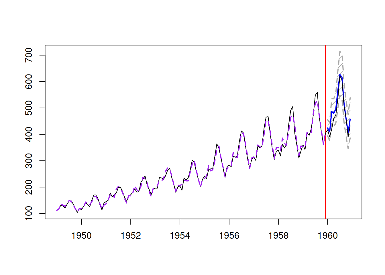
Figure 6.4: Forecast for air passengers data using an ETS(M,M,M) model.
If we want to calculate the error measures based on the conditional expectation, we can use the measures() function from the greybox package in the following way:
##           ME          MAE          MSE          MPE         MAPE          sCE         sMAE         sMSE         MASE
## -25.29641012  25.29641012 873.19440441  -0.05280830   0.05280830  -1.15644069   0.09637006   0.01267294   1.05034223
##        RMSSE         SAME         rMAE        rRMSE         rAME    asymmetry         sPIS
##   0.94311699   1.05034223   0.33284750   0.28695725   0.35545307  -1.00000000   7.49293853
These can be compared with the measures from the ETS(A,A,A) model:
##            ME           MAE           MSE           MPE          MAPE           sCE          sMAE          sMSE
##   3.837510534  13.028394826 283.477244757   0.004976399   0.027236387   0.175434116   0.049633413   0.004114193
##          MASE         RMSSE          SAME          rMAE         rRMSE          rAME     asymmetry          sPIS
##   0.540957123   0.537364781   0.159338789   0.171426248   0.163501157   0.053922865   0.415415558  -0.532467332
Comparing, for example, MSE from the two models, we can conclude that the pure additive one is more accurate than the pure multiplicative one, which could have happened purely by chance (we should do rolling origin to confirm this).
We can also produce the plot of the time series decomposition according to ETS(M,M,M) (see Figure 6.5):
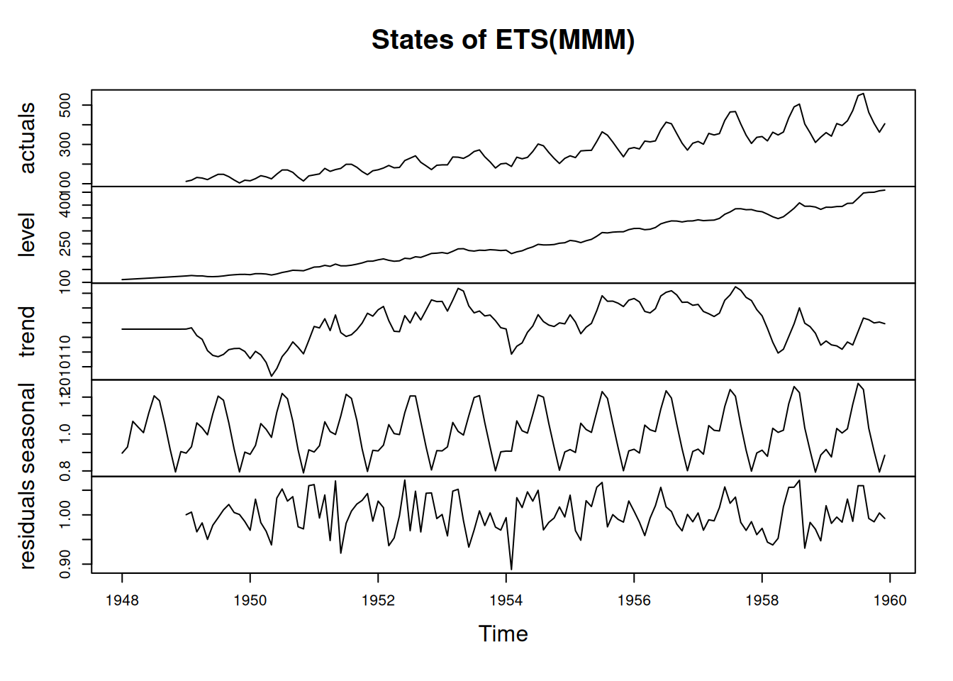
Figure 6.5: Decomposition of air passengers data using an ETS(M,M,M) model.
The plot in Figure 6.5 shows that the residuals are more random for the pure multiplicative model than for the ETS(A,A,A), but there still might be some structure left. The autocorrelation and partial autocorrelation functions (discussed in Section 8.3) might help in understanding this better:
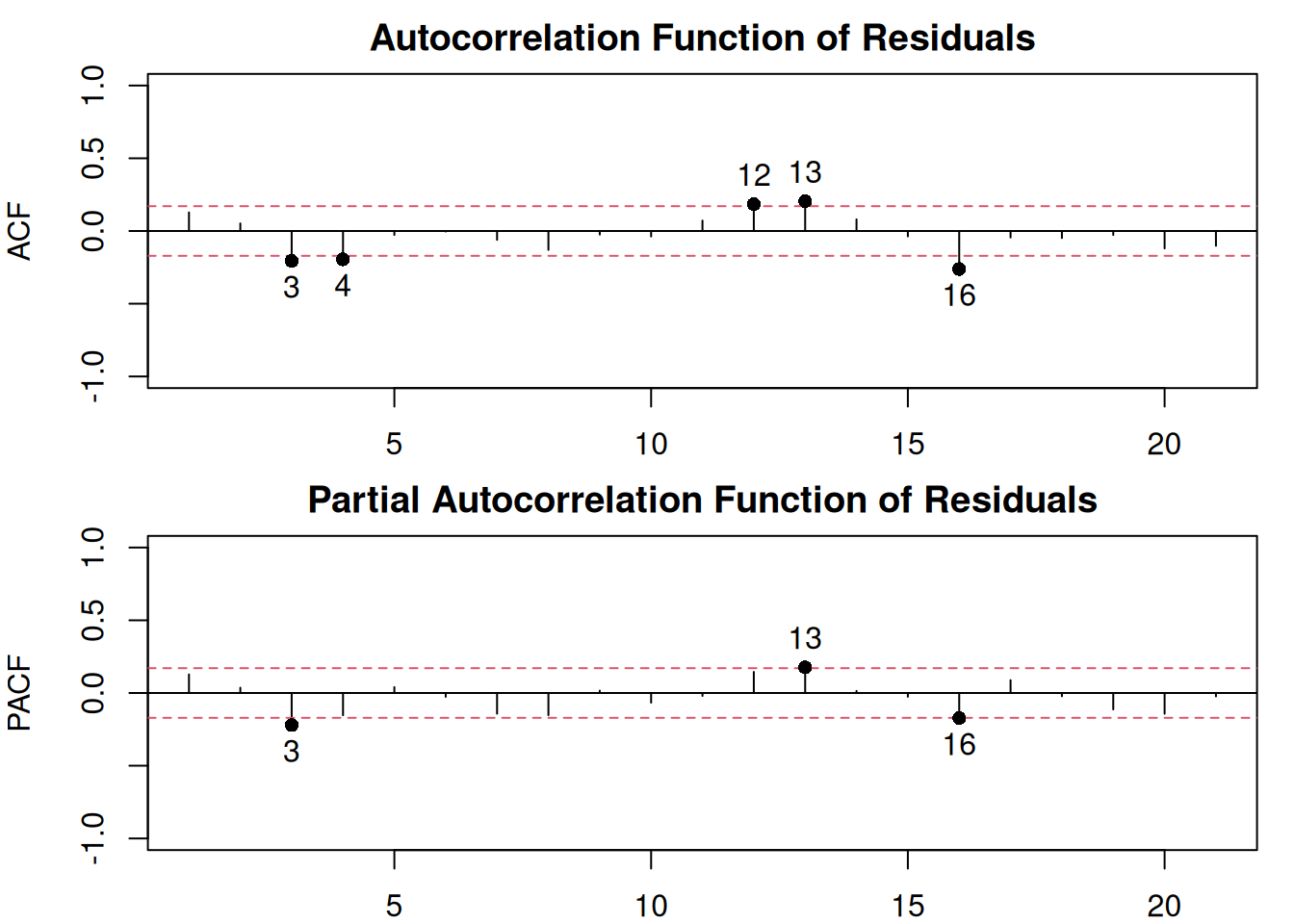
Figure 6.6: ACF and PACF of residuals of an ETS(M,M,M) model.
The plot in Figure 6.6 shows that there is still some correlation left in the residuals, which could be either due to pure randomness or imperfect estimation of the model. Tuning the parameters of the optimiser or selecting a different model might solve the problem.
The software behind this book. The methods described here are implemented in the smooth and greybox packages for R and Python, which are free and open source.
Want to learn this with us? We teach these methods to practitioners on Demand Forecasting Principles, a four-week online course, and run other courses in forecasting, statistics and analytics.