14.4 Model specification: Outliers
In statistics, it is assumed that if the model is correctly specified then it does not have influential outliers. This means that there are no observations that cannot be explained by the model and the variability around it. If they happen then this might mean that:
- We missed some important information (e.g. promotion) and did not include a respective variable in the model;
- There was an error in recordings of the data, e.g. a value of 2000 was recorded as 200;
- We did not miss anything predictable, we just face a distribution with fat tails (i.e. we assumed a wrong distribution).
In any of these cases, outliers might impact estimates of parameters of our model. With ETS, this might lead to higher than needed smoothing parameters, which in turn results in wider than needed prediction intervals and potentially biased forecasts. In the case of ARIMA, the mechanism is more complicated, still usually leading to widened intervals and biased forecasts. Finally, in regression, they might lead to biased estimates of parameters. So, it is important to identify outliers and deal with them.
14.4.1 Outliers detection
While it is possible to do preliminary analysis of the data and analyse distribution of the variable of interest, this does not allow identifying the outliers. This is because the simple univariate analysis (e.g. using boxplots) assumes that the variable has a fixed mean and a fixed distribution. This is violated by any model which has either a dynamic element or explanatory variables in it. So, the detection should be done based on residuals of an applied model.
One of the simplest ways of identifying outliers relies on distributional assumptions about the residuals and/or the response variable. For example, if we assume that our data follows the Normal distribution, we would expect 95% of observations to lie inside the bounds with approximately \(\pm 1.96\sigma\) and 99.8% of them to lie inside the \(\pm 3.09 \sigma\). Sometimes these values are substituted by heuristics “values lying inside 2/3 sigmas”, which is not precise and works only for Normal distribution. Still, based on this, we could flag the values outside these bounds and investigate them to see if any of them are indeed outliers.
Remark. If some observations lie outside these bounds, they are not necessarily outliers: building a 95% confidence interval always implies that approximately 5% of observations will lie outside the bounds.
Given that the ADAM supports different distributions, the heuristics mentioned above in general is inappropriate. We need to get proper quantiles for each of the assumed distributions. Luckily, this is not difficult because the quantile functions for all the distributions supported by ADAM either have analytical forms or can be obtained numerically.
Here is an example in R with the same multiplicative ETSX model and the standardised residuals vs fitted values with the 95% bounds (Figure 14.12):
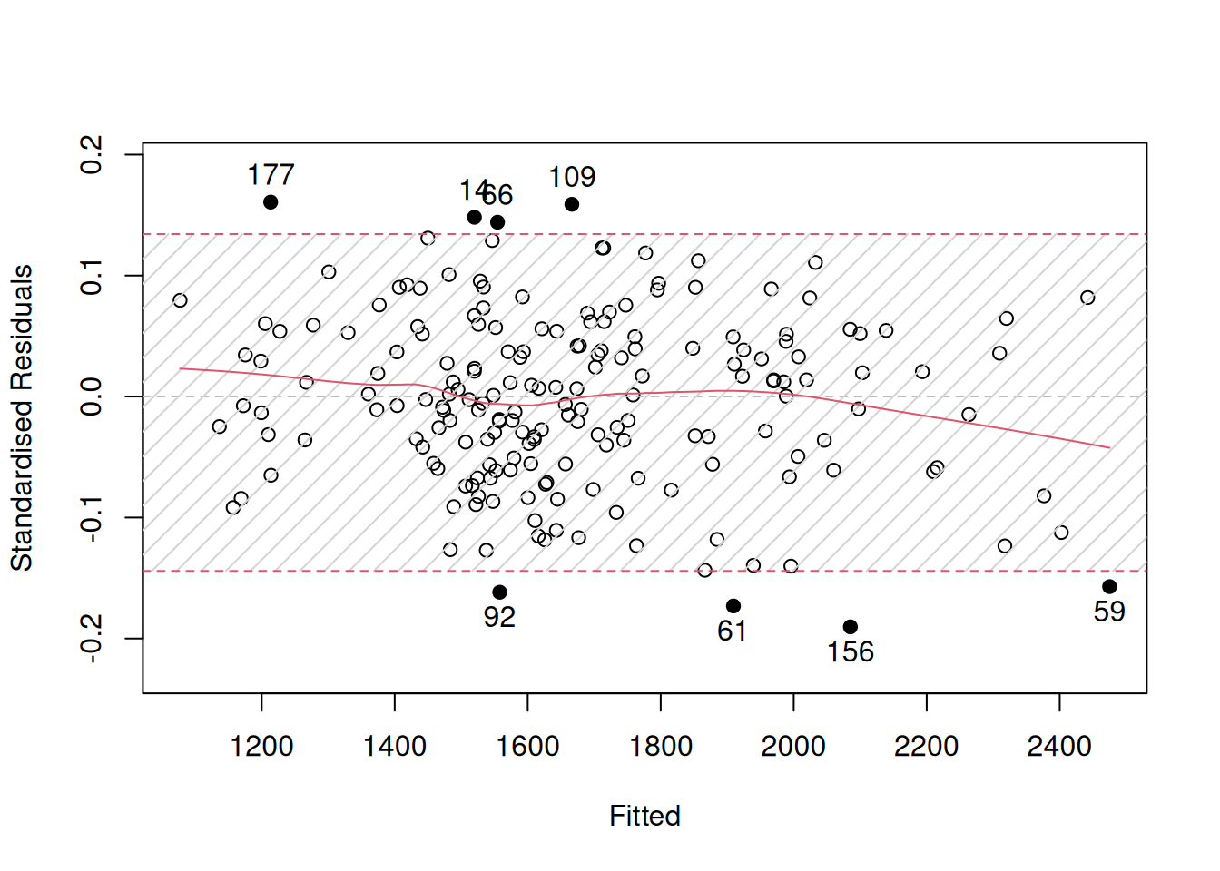
Figure 14.12: Standardised residuals vs fitted for the pure multiplicative ETSX model.
Remark. In the case of Inverse Gaussian, Gamma, and Log-Normal distributions, the function will produce the residuals in logarithms to make the plot more readable.
The plot in Figure 14.12 demonstrates that there are outliers, some of which are further away from the bounds. Although the amount of outliers is not large (it is roughly 5% of our sample), it would make sense to investigate why they happened.
Given that we deal with time series, plotting residuals vs time is also sometimes helpful (Figure 14.13):
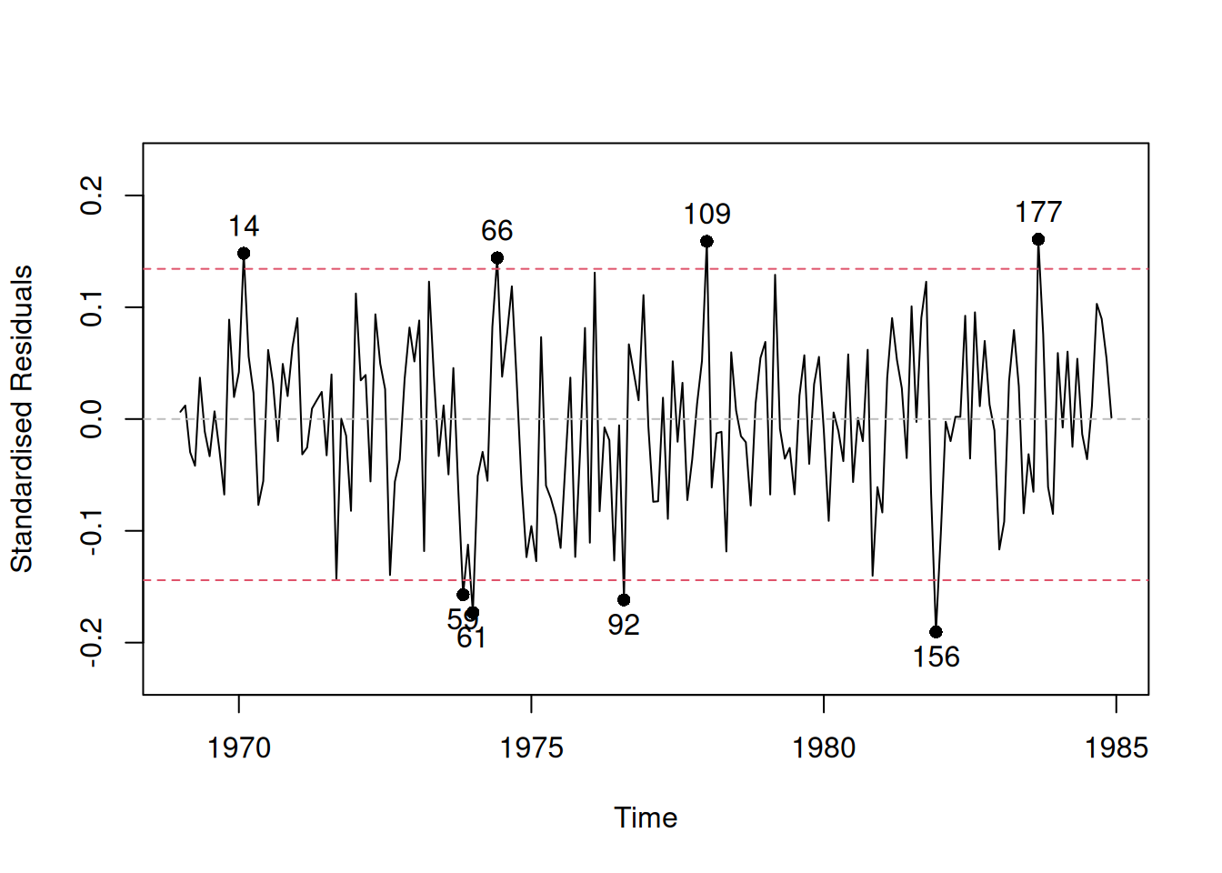
Figure 14.13: Standardised residuals vs time for the pure multiplicative ETSX model.
We see in Figure 14.13 that there is no specific pattern in the outliers, they happen randomly, so they appear not because of the omitted variables or wrong transformations. We have nine observations lying outside the bounds, which means that the 95% interval contains \(\frac{192-9}{192} \times 100 \% \approx 95.3 \%\) of observations (192 is the sample size). This is close to the nominal value.
In some cases, the outliers might impact the scale of distribution and will lead to wrong standardised residuals, distorting the picture. This is where studentised residuals come into play. They are calculated similarly to the standardised ones, but the scale of distribution is recalculated for each observation by considering errors on all but the current observation. So, in a general case, this is an iterative procedure that involves looking through \(t=\{1,\dots,T\}\) and that should, in theory, guarantee that the real outliers do not impact the scale of distribution. This procedure is simplified for the Normal distribution and has an analytical solution. We do not discuss it in the context of ADAM. Here is how they can be analysed in R:
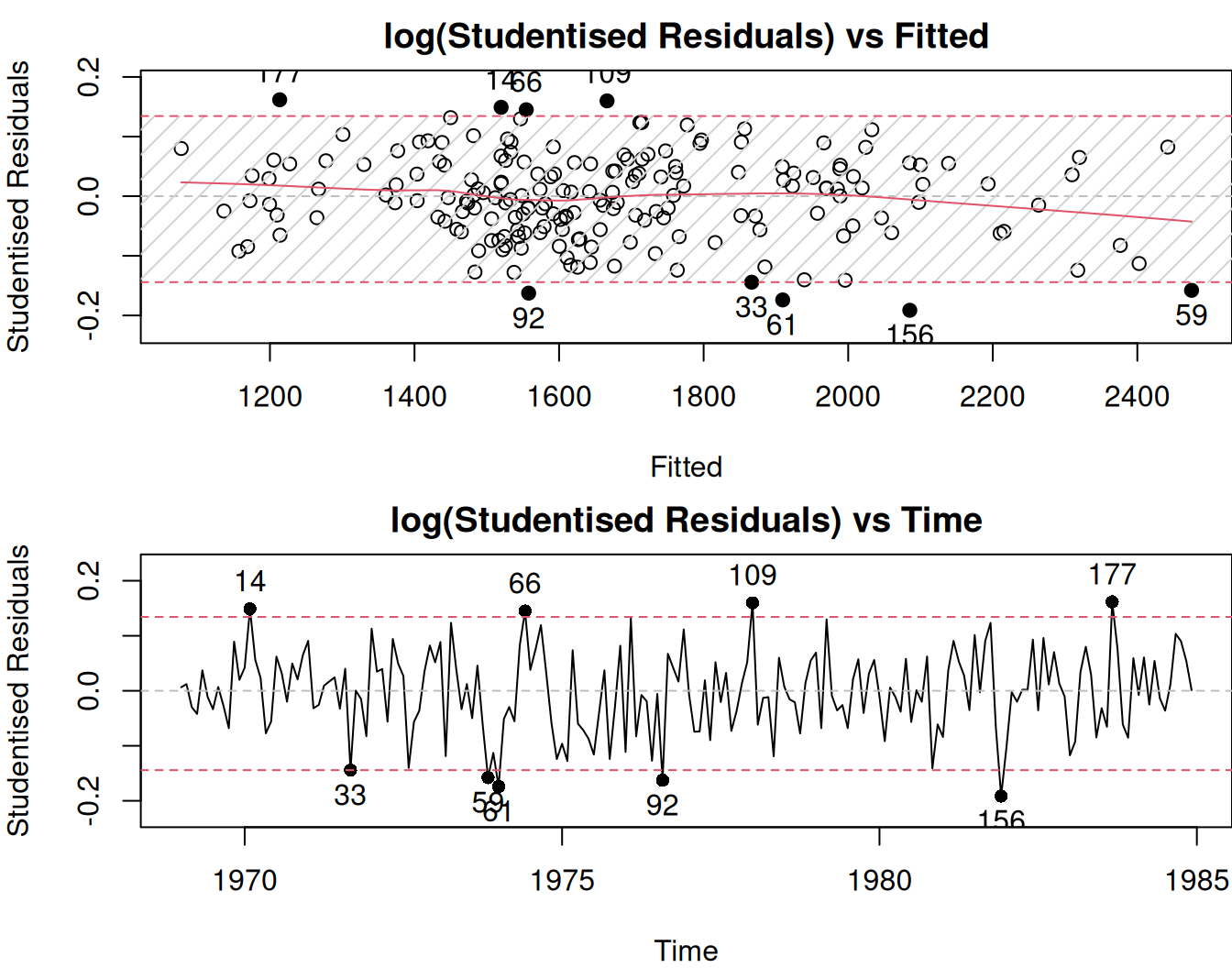
Figure 14.14: Studentised residuals analysis for the pure multiplicative ETSX model.
In many cases (ours included), the standardised and studentised residuals will look very similar. But in some cases of extreme outliers, they might differ, and the latter might show outliers better than the former.
Given the situation with outliers in our case, we could investigate when they happen in the original data to understand better whether they need to be taken care of. But instead of manually recording which of the observations lie beyond the bounds, we can get their ids via the outlierdummy() method from the greybox package, which extracts either standardised or studentised residuals (depending on what we want) and flags those observations that lie outside the constructed interval, automatically creating dummy variables for these observations. Here is how it works:
The method returns several objects (see the documentation for details), including the ids of outliers:
## [1] 14 59 61 66 92 109 156 177These ids can be used to produce additional plots. For example:
# Plot actuals
plot(actuals(adamSeat05), main="",
     ylab="Drivers injured")
# Add fitted
lines(fitted(adamSeat05),col="grey")
# Add points for the outliers
points(time(Seatbelts)[adamSeat05Outliers$id],
       Seatbelts[adamSeat05Outliers$id,"drivers"],
       col="red", pch=16)
# Add the text with ids of outliers
text(time(Seatbelts)[adamSeat05Outliers$id],
     Seatbelts[adamSeat05Outliers$id,"drivers"],
     adamSeat05Outliers$id, col="red", pos=2)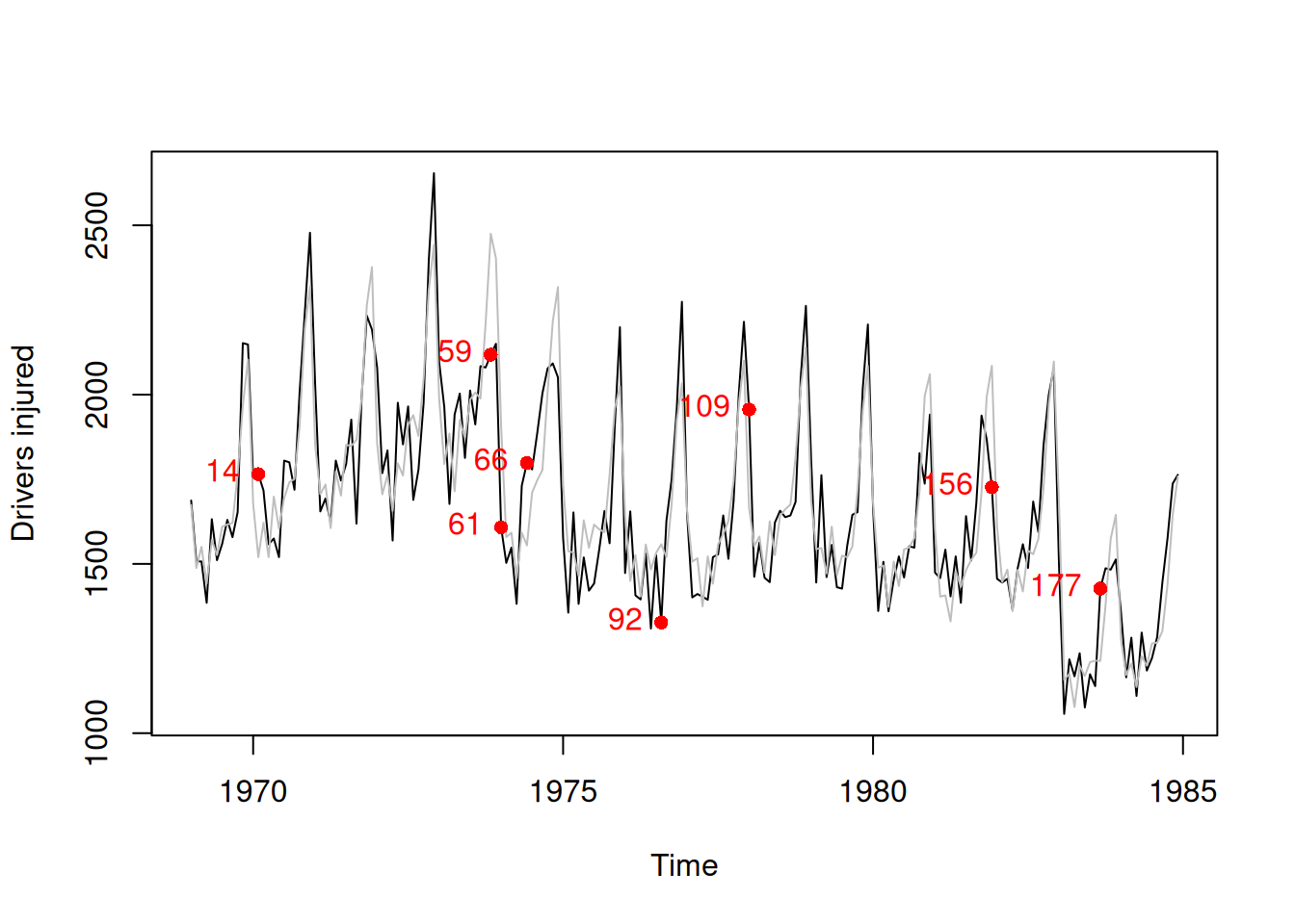
Figure 14.15: Actuals over time with points corresponding to outliers of the pure multiplicative ETSX model.
We cannot see any peculiarities in the appearance of outliers in Figure 14.15. They seem to happen at random. There might be some external factors, leading to those unexpected events (for example, the number of injuries being much lower than expected on observation 156, in November 1981), but investigation of these events is outside of the scope of this demonstration.
Remark. As a side note, in R, there are several methods for extracting residuals:
resid()orresiduals()will extract either \(e_t\) or \(1+e_t\), depending on the error type in the model;rstandard()will extract the standardised residuals \(u_t\);rstudent()will do the same for the studentised ones.
The smooth package also introduces the rmultistep function, which extracts multiple steps ahead in-sample forecast errors. We do not discuss this method here, but we will return to it in Subsection 14.7.3.
14.4.2 Dealing with outliers
While in the case of cross-sectional data some of the observations with outliers can be removed without damaging the model, in the case of time series, this is usually not possible to do. If we remove an observation from time series then we break its structure, and the applied model will not work as intended. So, we need to do something different to either interpolate the outliers or to tell the model that they happen.
Based on the output of the outlierdummy() method from the previous example, we can construct a model with explanatory variables to diminish the impact of outliers on the model:
# Add outliers to the data
SeatbeltsWithOutliers <-
    cbind(as.data.frame(Seatbelts[,-c(1,3,4,7)]),
          adamSeat05Outliers$outliers)
# Transform the drivers variable into time series object
SeatbeltsWithOutliers$drivers <- ts(SeatbeltsWithOutliers$drivers,
                                    start=start(Seatbelts),
                                    frequency=frequency(Seatbelts))
# Run the model with all the explanatory variables in the data
adamSeat06 <- adam(SeatbeltsWithOutliers, "MNM", lags=12,
                   formula=drivers~.)
In order to decide, whether the dummy variables help or not, we can use information criteria, comparing the two models:
##         ETSX ETSXOutliers
##     2385.812     2363.520
Comparing the two values above, we would conclude that adding dummies improves the model. However, this could be a mistake, given that we do not know the reasons behind most of them. In general, we should not include dummy variables for the outliers unless we know why they happened. If we do that, we might overfit the data. Still, if we have good reasons for this, we could add explanatory variables for outliers in the function to remove their impact on the response variable.
14.4.3 An automatic mechanism
An automated mechanism based on what we have done manually in the previous subsection, is implemented in the adam() function, which has the outliers parameter, defining what to do with them if there are any with the following three options:
"ignore"– do nothing;"use"– create the model with explanatory variables including all of them, as shown in the previous subsection, and see if it is better than the model without the variables in terms of an information criterion;"select"– create lags and leads of dummies fromoutlierdummy()and then select the dummies based on the explanatory variables selection mechanism (discussed in Section 15.3). Lags and leads are needed for cases when the effect of outliers is carried over to neighbouring observations.
Here is how this works in our case:
adamSeat08 <- adam(Seatbelts, "MNM", lags=12,
                   formula=drivers~PetrolPrice+kms+law,
                   outliers="select", level=0.95)
AICc(adamSeat08)
## [1] 2394.344This model has selected some dummies for outliers. We can see them by looking at the coefficients of the model:
##         alpha         gamma      outlier7      outlier8      outlier6
##    0.39168620    0.04095824   -0.18129627    0.12989137    0.15447026
##      outlier4      outlier1      outlier2      outlier3      outlier5
##    0.10298678    0.12503198   -0.08320828   -0.13449400   -0.15667998
##  outlier2Lag1  outlier5Lag1 outlier4Lead1
##   -0.11574144    0.02553479    0.03970096
Given that this is an automated approach, it is prone to potential mistakes. It needs to be treated with care as it might select unnecessary dummy variables and lead to overfitting. I would recommend exploring the outliers manually when possible and not relying too much on the automated procedures.
14.4.4 Final remarks
Koehler et al. (2012) explored the impact of outliers on ETS performance in terms of forecasting accuracy. They found that if outliers happen at the end of the time series, it is important to take them into account in a model. If they happen much earlier, their impact on the final forecast will be negligible. Unfortunately, the authors did not explore the impact of outliers on the prediction intervals. Based on my experience, I can tell that the outliers typically impact the width of the interval rather than the point forecasts. So, it is important to take care of them when they happen.