1.3 Types of forecasts
Depending on circumstances, we might require different types of forecasts with different characteristics. It is essential to understand what your model produces to measure its performance correctly (see Section 2.1) and make correct decisions in practice. Several things are typically produced for forecasting purposes. We start with the most common one.
1.3.1 Point forecasts
Point forecast is the most often produced type of forecast. It corresponds to a trajectory from a model. This, however, might align with different types of statistics depending on the model and its assumptions. In the case of a pure additive model (such as linear regression), the point forecasts correspond to the conditional expectation (mean) from the model. The conventional interpretation of this value is that it shows what to expect on average if the situation would repeat itself many times (e.g. if we have the day with similar conditions, then the average temperature will be 10 degrees Celsius). In the case of time series, this interpretation is difficult to digest, given that time does not repeat itself, but this is the best we have. We will come back to the technicalities of producing conditional expectations from ADAM in Section 18.2.
Another type of point forecast is the (conditional) geometric expectation (geometric mean). It typically arises, when the model is applied to the data in logarithms and the final forecast is then exponentiated. This becomes apparent from the following definition of geometric mean: \[\begin{equation} \check{\mu} = \sqrt[T]{\prod_{t=1}^T y_t} = \exp \left(\frac{1}{T} \sum_{t=1}^T \log(y_t) \right) , \tag{1.1} \end{equation}\] where \(y_t\) is the actual value on observation \(t\), and \(T\) is the sample size. To use the geometric mean, we need to assume that the actual values can only be positive. Otherwise, the root in (1.1) might produce imaginary units (because of taking a square root of a negative number) or be equal to zero (if one of the values is zero). In general, the arithmetic and geometric means are related via the following inequality: \[\begin{equation} \check{\mu} \leq \mu , \tag{1.2} \end{equation}\] where \(\check{\mu}\) is the geometric mean and \(\mu\) is the arithmetic one. Although geometric mean makes sense in many contexts, it is more difficult to explain than the arithmetic one to decision makers.
Finally, sometimes medians are used as point forecasts. In this case, the point forecast splits the sample into two halves and shows the level below which 50% of observations will lie in the future.
Remark. The specific type of point forecast will differ depending on the model used in construction. For example, in the case of the pure additive model, assuming some symmetric distribution (e.g. Normal one), the arithmetic mean, geometric mean, and median will coincide. On the other hand, a model constructed in logarithms will assume an asymmetric distribution for the original data, leading to the following relation between the means and the median (in case of positively skewed distribution): \[\begin{equation} \begin{aligned} & \check{\mu} \leq \mu \\ & \tilde{\mu} \leq \mu \end{aligned} , \tag{1.3} \end{equation}\] where \(\tilde{\mu}\) is the median of distribution. The relation between geometric mean and median is more complicated and will differ from one distribution to another. In case of symmetric distributions or distributions becoming symmetric in logarithms, the two measures should coincide (at least in theory).
1.3.2 Quantiles and prediction intervals
As some forecasters say, all point forecasts are wrong. They will never correspond to the actual values because they only capture the model’s mean (or median) performance, as discussed in the previous subsection. Everything that is not included in the point forecast can be considered as the uncertainty of demand. For example, we never will be able to say precisely how many cups of coffee a cafe will sell on the forthcoming Monday, but we can at least capture the main tendencies and the uncertainty around our point forecast.
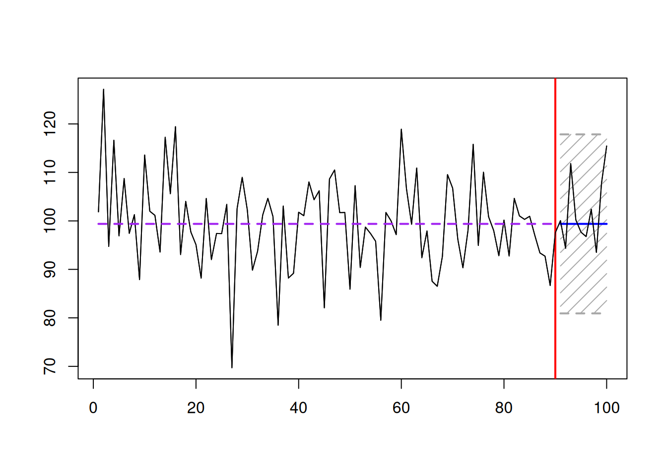
Figure 1.1: An example of a well-behaved data, point forecast, and a 95% prediction interval.
Figure 1.1 shows an example with a well-behaved demand, for which the best point forecast is the straight line. To capture the uncertainty of demand, we can construct the prediction interval, which will tell roughly where the demand will lie in \(1-\alpha\) percent of cases. The interval in Figure 1.1 has the width of 95% (significance level \(\alpha=0.05\)) and shows that if the situation is repeated many times, the actual demand will be between 80.92 and 117.85. Capturing the uncertainty correctly is important because real-life decisions need to be made based on the full information, not only on the point forecasts.
We will discuss how to produce prediction intervals in more detail in Section 18.3. For a more detailed discussion on the concepts of prediction and confidence intervals, see Chapter 6 of Svetunkov and Yusupova (2025).
Another way to capture the uncertainty (related to the prediction interval) is via specific quantiles of distribution. The prediction interval typically has two sides, leaving \(\frac{\alpha}{2}\) values outside of each side of distribution. Instead of producing the interval, in some cases, we might need just a specific quantile, essentially creating the one-sided prediction interval (see Section 18.4.2 for technicalities). The bound in this case will show the particular value below which the pre-selected percentage of cases would lie. This becomes especially useful in such contexts as the safety stock calculation (because we are not interested in knowing the lower bound, we want products in inventory to satisfy some proportion of demand).
1.3.3 Forecast horizon
Finally, an important aspect in forecasting is the horizon, for which we need to produce forecasts. Depending on the context, we might need:
- Only a specific value h steps ahead, e.g., the temperature following Monday.
- All values from 1 to h steps ahead, e.g. how many patients we will have each day next week.
- Cumulative values for the period from 1 to h steps ahead, e.g. what the cumulative demand over the lead time (the time between the order and product delivery) will be (see discussion in Section 18.4.3).
It is essential to understand how decisions are made in practice and align them with the forecast horizon. In combination with the point forecasts and prediction intervals discussed above, this will give us an understanding of what to produce from the model and how. For example, in the case of safety stock calculation, it would be more reasonable to produce quantiles of the cumulative over the lead time demand than to produce point forecasts from the model (see, for example, discussion on safety stock calculation in Silver et al., 2016).