14.6 Residuals are i.i.d.: Heteroscedasticity
Another important assumption for conventional models is that the residuals are homoscedastic, meaning that their variance stays the same (no matter what). If it does not then the parameters of the model might be inefficient (thus change substantially with the change of the sample size) and prediction intervals from the model might be miscalibrated (either narrower or wider than needed, depending on the circumstances). This section will show how the issue can be diagnosed and resolved.
14.6.1 Detecting heteroscedasticity
Building upon our previous example, we will use the ETSX(A,N,A) model, which has some issues, as we remember from Section 14.3. One of those is the wrong type of model – additive instead of multiplicative. This is also related to the variance of residuals, because the multiplicative error model takes care of one of the types of heteroscedasticity. To see if the residuals of the ETSX(A,N,A) model are homoscedastic, we can plot them against the fitted values (Figure 14.21):
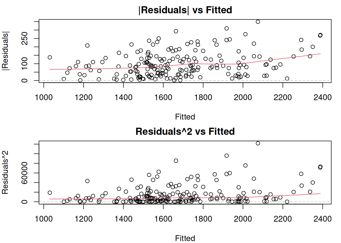
Figure 14.21: Absolute and squared residuals vs fitted of Model 3.
The two plots in Figure 14.21 allow detecting a specific type of heteroscedasticity when the residuals’ variability changes with the increase of fitted values. The plot of absolute residuals vs fitted is more appropriate for models, where the scale parameter is calculated based on absolute values of residuals (e.g. the model with Laplace distribution) and relates to MAE (Subsection 11.2.1), while the squared residuals vs fitted shows whether the variance of residuals is stable or not (thus making it more suitable for models with Normal and related distributions). However, the squared residuals plot might be challenging to read due to outliers, so the first one might help detect the heteroscedasticity even when the scale is supposed to rely on squared errors. What we want to see on these plots is for all the points to lie in the same corridor for lower and for the higher fitted values and for the red LOWESS line to be parallel to the x-axis. In our case, there is a slight increase in the line. Furthermore, the variability of residuals around 1000 is lower than the one around 2000, indicating that we have heteroscedasticity in residuals. In our case, this is caused by the wrong transformations in the model (see Section 14.3), so to fix the issue, we should switch to a multiplicative model. In fact, switching to a multiplicative model (aka model in logarithms) fixes the heteroscedasticity issue in many cases in practice.
Another diagnostics tool that might become useful in some situations is the plot of absolute and squared standardised residuals versus fitted values. They have a similar idea to the previous plots, but they might change slightly because of the standardisation (mean is equal to 0 and scale is equal to 1). These plots become especially useful if the changing variance is modelled explicitly (e.g. via a regression model or a GARCH-type of model, I will discuss this in Chapter 17):
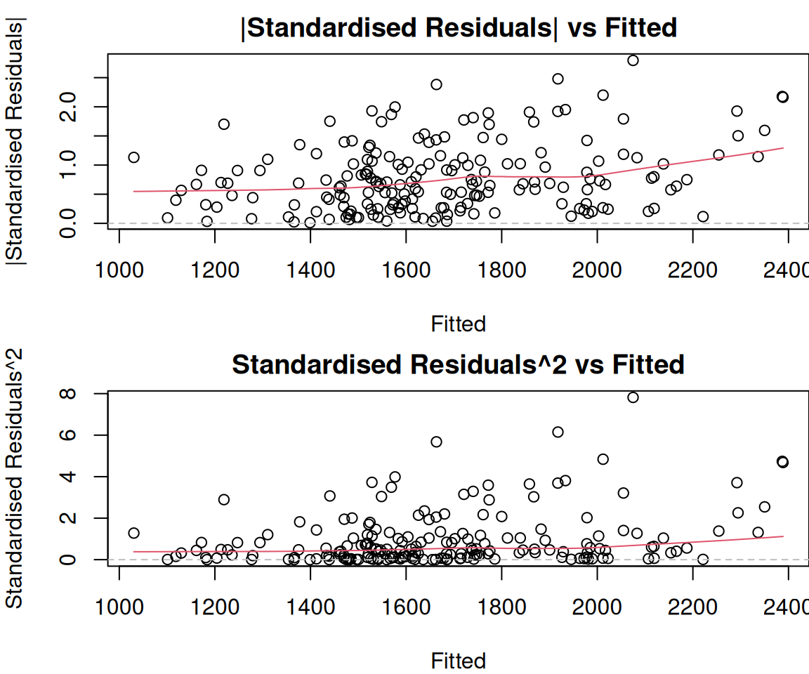
Figure 14.22: Absolute and squared standardised residuals vs fitted of Model 3.
In our case, the plots in Figure 14.22 do not give an additional message. We already know that there is a slight heteroscedasticity and that we need to transform the response variable.
If we suspect that there are some specific variables that might cause heteroscedasticity, we can plot absolute or squared residuals vs these variables to see if they indeed cause it. For example, here is how we can produce a basic plot of absolute residuals vs all explanatory variables included in the model:
cbind(as.data.frame(abs(resid(adamSeat03))),
      adamSeat03$data[,all.vars(formula(adamSeat03))[-1]]) |>
    spread(LOWESS=TRUE)
Figure 14.23: Spread plot of absolute residuals vs variables included in Model 3.
The plot in Figure 14.23 can be read similarly to the plots discussed above: if we notice a change in variability of residuals or a change (increase or decrease) in the LOWESS lines with the change of a variable, then this might indicate that the respective variable causes heteroscedasticity. In our example, it looks like the variable law causes the most significant issue – all the other variables do not cause as substantial a change in the variance as this one. If we want to fix this specific issue then we might need to consider a scale model, modelling the change of scale based on variables like law directly (this will be discussed in Chapter 17).
We already know that we need to use a multiplicative model instead of the additive one in our example, so we will see how the residuals look for the correctly specified model in Figure 14.24.
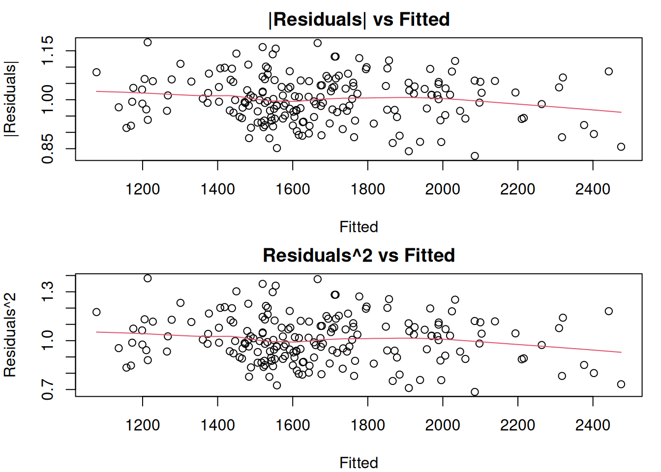
Figure 14.24: Absolute and Squared residuals vs Fitted of Model 5.
The plots in Figure 14.24 do not demonstrate any substantial issues: the residuals look homoscedastic, and given the scale of residuals, the change of LOWESS line does not reflect significant changes in the scale of the residuals. An additional plot of absolute residuals vs explanatory variables does not show any severe issues either (Figure 14.25). So, we can conclude that the multiplicative model resolves the issue with heteroscedasticity.
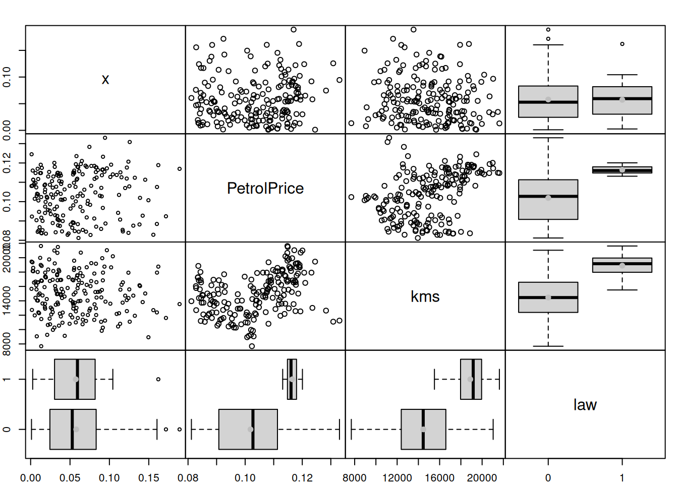
Figure 14.25: Spread plot of absolute residuals vs variables included in the Model 5.
Concluding this section, we have focused the analysis on the visual diagnostics. But there are formal statistical tests for heteroscedasticity, such as White (White, 1980), Breusch-Pagan (Breusch and Pagan, 1979), and Bartlett’s (Bartlett, 1937) tests and others. They all test different types of heteroscedasticity and can be used when the visual diagnostics are not possible. We do not discuss them here for a reason outlined in Section 14.5.