15.4 Forecasts combinations
When it comes to achieving the most accurate forecasts possible in practice, the most robust (in terms of not failing) approach is producing combined forecasts. The primary motivation for combining is that there is no one best forecasting method for everything – methods might perform very well in some conditions and fail in others. It is typically not possible to say which of the cases you face in practice. Furthermore, the model selected on one sample might differ from the model chosen for the same sample but with one more observation. Thus there is a model uncertainty (as defined by Chatfield, 1996), which can be mitigated by producing forecasts from several models and then combining them to get the final forecast. This way, the potential damage from an inaccurate forecast is typically reduced.
There are many different techniques for combining forecasts. The non-exhaustive list includes:
- Simple average, which works fine as long as you do not have exceptionally poorly performing methods;
- Median, which produces good combinations when the pool of models is relatively small and might contain those that produce very different forecasts from the others (e.g. explosive trajectories). However, when a big pool of models is considered, the median might ignore vital information and decrease accuracy, as noted by Jose and Winkler (2008). Stock and Watson (2004) conducted an experiment on macroeconomic data, and medians performed poorer than the other approaches (probably because of the high number of forecasting methods), while a median-based combination worked well for Petropoulos and Svetunkov (2020), who considered only four forecasting approaches;
- Trimmed and/or Winsorized mean, which drop extreme forecasts, when calculating the mean and, as was shown by Jose and Winkler (2008), work well in cases of big pools of models, outperforming medians and simple average;
- Weighted mean, which assigns weights to each forecast and produces a combined forecast based on them. While this approach sounds more reasonable than the others, there is no guarantee that it will work better because the weights need to be estimated and might change with the change of sample size or a pool of models. Claeskens et al. (2016) explain why the simple average approach outperforms weighted averages in many cases: it does not require estimation of weights and thus does not introduce as much uncertainty. However, when done smartly, combinations can be beneficial in terms of accuracy, as shown, for example, by Kolassa (2011) and Kourentzes et al. (2019a).
The forecast combination approach implemented in ADAM is the weighted mean, based on Kolassa (2011), who used AIC weights as proposed by Burnham and Anderson (2004). This approach aims to estimate all models in the pool, calculate information criteria for each of them (see discussion in Section 16.4 in Svetunkov and Yusupova, 2025) and then calculate weights for each model. Those models with lower ICs will have higher weights, while the poorly performing ones will have the lower ones. The only requirement of the approach is for the parameters of models to be estimated via likelihood maximisation (see Section 11.1). Furthermore, it is not important what model is used or what distribution is assumed, as long as the models are initialised (see discussion in Section 11.4) and constructed in the same way and the likelihood is used in the estimation.
When it comes to prediction intervals, the correct way of calculating them for the combination is to consider the joint distribution of all forecasting models in the pool and take quantiles based on that. However, Lichtendahl et al. (2013) showed that a simpler approach of averaging the quantiles works well in practice. This approach implies producing prediction intervals for all the models in the pool and then averaging the obtained values. It is fast and efficient in terms of getting prediction intervals from a combined model.
In R, the adam() function supports the combination of ETS models via model="CCC" or any other combination of letters, as long as the model contains “C” in its name. For example, the function will combine all non-seasonal models if model="CCN" is provided. Consider the following example on Box-Jenkins sales series:
In the code above, the function will estimate all non-seasonal models, extract AICc for each of them and then calculate weights, which we can be extracted for further analysis:
##   ANN   MAN  AAdN   MMN  AMdN   MNN   AAN  MAdN   AMN  MMdN
## 0.000 0.010 0.392 0.007 0.416 0.000 0.054 0.043 0.033 0.046
As can be seen from the output of weights, the level models ETS(A,N,N) and ETS(M,N,N) were further away from the best model and, as a result, got weights very close to zero.
In the ADAM combination, the fitted values are combined from all models, while the residuals are calculated as \(e_t = y_t -\hat{y}_t\), where \(\hat{y}_t\) is the combined value. The final forecast together with the prediction interval can be generated via the forecast() function (Figure 15.2):
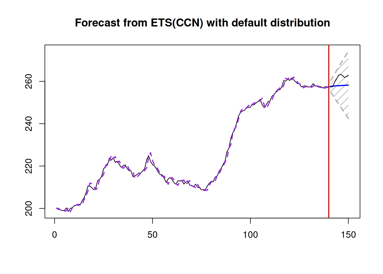
Figure 15.2: An example of a combination of ETS non-seasonal models on Box-Jenkins sale time series.
What the function above does, in this case, is produces forecasts and prediction intervals from each model and then uses original weights to combine them. Each model can be extracted and used separately if needed. Here is an example with the ETS(A,Ad,N) model from the estimated pool:
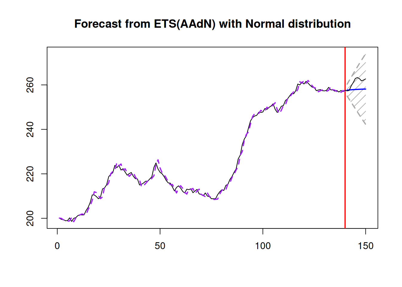
Figure 15.3: An example of the combination of ETS non-seasonal models on Box-Jenkins sale time series.
As can be seen from the plots in Figures 15.2 and 15.3, due to the highest weight, ETS(A,Ad,N) and ETS(C,C,N) models have produced very similar point forecasts and prediction intervals.
Alternatively, if we do not need to consider all ETS models, we can provide the pool of models, including a model with “C” in its name. Here is an example of how pure additive non-seasonal models can be combined:
The main issue with the combined ETS approach is that it is computationally expensive due to the estimation of all models in the pool and can also result in high memory usage (because it saves all the estimated models). As a result, it is recommended to be smart in deciding which models to include in the pool.
15.4.1 Other combination approaches
While adam() supports information criterion weights combination of ETS models only, it is also possible to combine ARIMA, regression models, and models with different distributions in the framework. Given that all models are initialised in the same way and that the likelihoods are calculated using similar principles, the weights can be calculated manually using the formula from Burnham and Anderson (2004):
\[\begin{equation}
w_i = \frac{\exp\left(-\frac{1}{2}\Delta_i\right)}{\sum_{j=1}^n \exp\left(-\frac{1}{2}\Delta_j\right)},
\tag{15.1}
\end{equation}\]
where \(\Delta_i=\mathrm{IC}_i -\min_{i=1}^n \left(\mathrm{IC}_i\right)\) is the information criteria distance from the best performing model, \(\mathrm{IC}_i\) is the value of an information criterion of model \(i\), and \(n\) is the number of models in the pool. For example, here how we can combine the best ETS with the best ARIMA and the ETSX(M,M,N) model in the ADAM framework, based on BICc:
# Prepare data with explanatory variables
BJsalesData <- cbind(as.data.frame(BJsales),
                     xregExpander(BJsales.lead,c(-5:5)))

# Apply models
adamPoolBJ <- vector("list",3)
adamPoolBJ[[1]] <- adam(BJsales, "ZZN",
                        h=10, holdout=TRUE,
                        ic="BICc")
adamPoolBJ[[2]] <- adam(BJsales, "NNN",
                        orders=list(ar=3,i=2,ma=3,select=TRUE),
                        h=10, holdout=TRUE,
                        ic="BICc")
adamPoolBJ[[3]] <- adam(BJsalesData, "MMN",
                        h=10, holdout=TRUE,
                        ic="BICc",
                        regressors="select")

# Extract BICc values
adamsICs <- sapply(adamPoolBJ, BICc)

# Calculate weights
adamsICWeights <- adamsICs - min(adamsICs)
adamsICWeights[] <- exp(-0.5*adamsICWeights) /
                    sum(exp(-0.5*adamsICWeights))
names(adamsICWeights) <- c("ETS","ARIMA","ETSX")
round(adamsICWeights, 3)
## ETS ARIMA ETSX
## 0.592 0.363 0.045These weights can then be used for the combination of the fitted values, forecasts, and prediction intervals:
# Produce forecasts from the three models
adamPoolBJForecasts <- lapply(adamPoolBJ, forecast,
                              h=10, interval="pred")

# Produce combined conditional means and prediction intervals
finalForecast <- cbind(sapply(adamPoolBJForecasts,
                              "[[","mean") %*% adamsICWeights,
                       sapply(adamPoolBJForecasts,
                              "[[","lower") %*% adamsICWeights,
                       sapply(adamPoolBJForecasts,
                              "[[","upper") %*% adamsICWeights)
# Give the appropriate names
colnames(finalForecast) <- c("Mean",
                             "Lower bound (2.5%)",
                             "Upper bound (97.5%)")
# Transform the table in the ts format (for convenience)
finalForecast <- ts(finalForecast,
                    start=start(adamPoolBJForecasts[[1]]$mean))
finalForecast
## Time Series:
## Start = 141
## End = 150
## Frequency = 1
## Mean Lower bound (2.5%) Upper bound (97.5%)
## 141 257.6656 254.9232 260.4382
## 142 257.7489 253.3927 262.0411
## 143 257.8307 251.9773 263.7050
## 144 257.9023 250.4785 265.3609
## 145 257.9759 248.9201 267.0322
## 146 258.0449 247.4410 268.6553
## 147 258.0981 245.9056 270.3768
## 148 258.1643 244.3623 272.1526
## 149 258.2186 242.8434 273.8260
## 150 258.2665 241.2664 275.5464In order to see how the forecast looks, we can plot it via graphmaker() function from greybox:
graphmaker(BJsales, finalForecast[,1],
           lower=finalForecast[,2], upper=finalForecast[,3],
           level=0.95)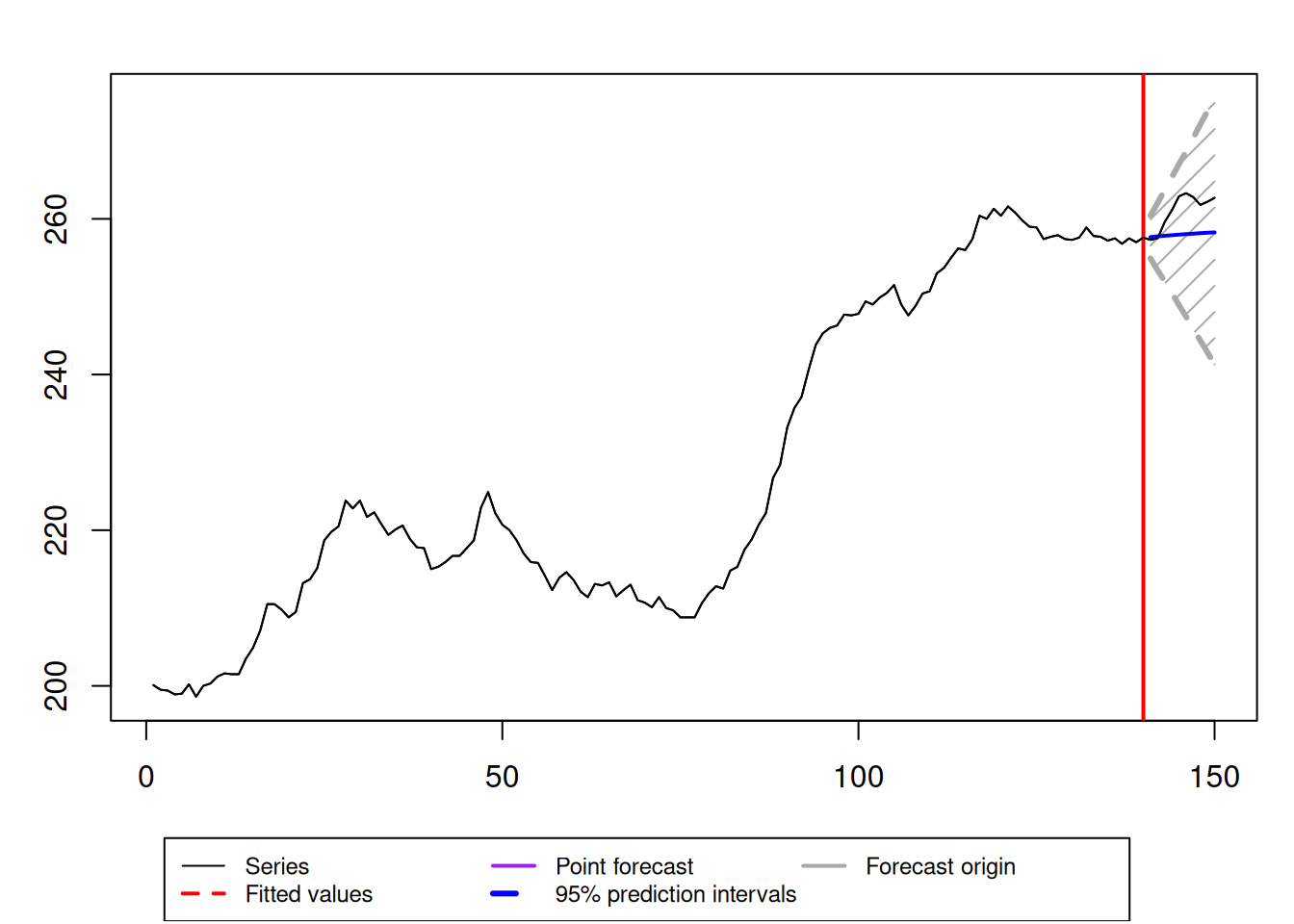
Figure 15.4: Final forecast from the combination of ETS, ARIMA, and ETSX models.
Figure 15.4 demonstrates the slightly increasing trajectory with an expanding prediction interval. The point forecast (conditional mean) continues the trajectory observed on the last several observations, just before the forecast origin. The future values are inside the prediction interval, so overall, this can be considered a reasonable forecast.