4.3 ETS and SES
Taking a step back, in this section we discuss one of the basic ETS models, the local level model, and the Exponential Smoothing method related to it.
4.3.1 ETS(A,N,N)
There have been several tries to develop statistical models underlying SES, and we know now that the model has underlying ARIMA(0,1,1) (Muth, 1960), local level MSOE (Multiple Source of Error, Muth, 1960) and SSOE (Single Source of Error, Snyder, 1985) models. According to Hyndman et al. (2002), the ETS(A,N,N) model also underlies the SES method. To see the connection and to get to it from SES, we need to recall two things: how in general, the actual value relates to the forecast error and the fitted value, and the error correction form of SES from Subsection 3.4.3: \[\begin{equation} \begin{aligned} & y_t = \hat{y}_{t} + e_t \\ & \hat{y}_{t+1} = \hat{y}_{t} + \hat{\alpha} e_{t} \end{aligned} . \tag{4.1} \end{equation}\] In order to get to the SSOE state space model for SES, we need to substitute \(\hat{y}_t=\hat{l}_{t-1}\), implying that the fitted value is equal to the level of the series: \[\begin{equation} \begin{aligned} & y_t = \hat{l}_{t-1} + e_t \\ & \hat{l}_{t} = \hat{l}_{t-1} + \hat{\alpha} e_{t} \end{aligned} . \tag{4.2} \end{equation}\] If we now substitute the sample estimates of level, smoothing parameter, and forecast error by their population values, we will get the ETS(A,N,N), which was discussed in Section 4.2: \[\begin{equation} \begin{aligned} & y_{t} = l_{t-1} + \epsilon_t \\ & l_t = l_{t-1} + \alpha \epsilon_t \end{aligned} , \tag{4.3} \end{equation}\] where, as we know from Section 3.1, \(l_t\) is the level of the data, \(\epsilon_t\) is the error term, and \(\alpha\) is the smoothing parameter. Note that we use \(\alpha\) without the “hat” symbol, which implies that there is a “true” value of the parameter (which could be obtained if we had all the data in the world or just knew it for some reason). The main benefit of having the model (4.3) instead of just the method (3.21) is in having a flexible framework, which allows adding other components, selecting the most appropriate ones (Section 15.1), consistently estimating parameters (Chapter 11), producing prediction intervals (Section 18.3), etc. In a way, this model is the basis of ADAM.
In order to see the data that corresponds to the ETS(A,N,N) we can use the sim.es() function from the smooth package. Here are several examples with different smoothing parameters values:
# list with generated data
y <- vector("list",6)
# Parameters for DGP
initial <- 1000
meanValue <- 0
sdValue <- 20
alphas <- c(0.1,0.3,0.5,0.75,1,1.5)
# Go through all alphas and generate respective data
for(i in 1:length(alphas)){
  y[[i]] <- sim.es("ANN", 120, 1, 12, persistence=alphas[i],
                   initial=initial, mean=meanValue, sd=sdValue)
}
The generated data can be plotted the following way:
par(mfrow=c(3,2), mar=c(2,2,2,1))
for(i in 1:6){
  plot(y[[i]], main=paste0("alpha=",y[[i]]$persistence),
       ylim=initial+c(-500,500))
}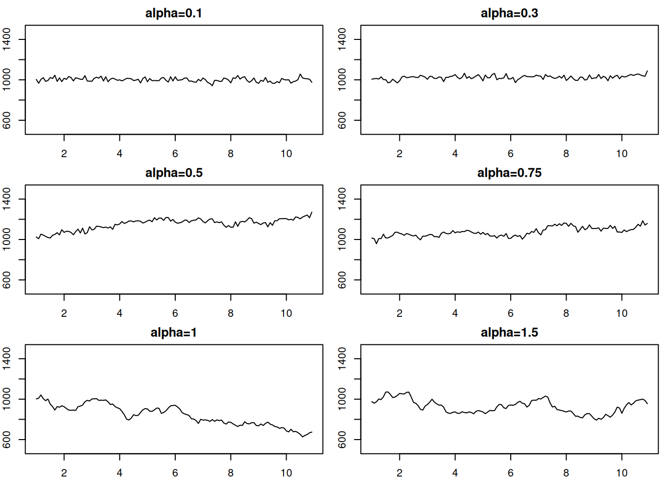
Figure 4.3: Local level data corresponding to the ETS(A,N,N) model with different smoothing parameters.
This simple simulation shows that the smoothing parameter in ETS(A,N,N) controls the variability in the data (Figure 4.3): the higher \(\alpha\) is, the higher variability is and less predictable the data becomes. With the higher values of \(\alpha\), the level changes faster, leading to increased uncertainty about the future values.
When it comes to the application of this model to the data, the conditional \(h\) steps ahead mean corresponds to the point forecast and is equal to the last observed level: \[\begin{equation} \mu_{y,t+h|t} = \hat{y}_{t+h} = l_{t} . \tag{4.4} \end{equation}\] This holds because it is assumed (see Section 1.4.1) that \(\mathrm{E}(\epsilon_t)=0\), which implies that the conditional \(h\) steps ahead expectation of the level in the model is (from the second equation in (4.3)): \[\begin{equation} \mathrm{E}(l_{t+h-1}|t) = l_t + \mathrm{E}(\alpha\sum_{j=1}^{h-2}\epsilon_{t+j}|t) = l_t . \tag{4.5} \end{equation}\]
Here is an example of a forecast from ETS(A,N,N) with automatic parameter estimation using the es() function from the smooth package:
# Generate the data
y <- sim.es("ANN", 120, 1, 12, persistence=0.3, initial=1000)
# Apply ETS(A,N,N) model
esModel <- es(y$data, "ANN", h=12, holdout=TRUE)
# Produce forecasts
esModel |> forecast(h=12, interval="pred") |>
    plot(main=paste0("ETS(ANN) with alpha=",
                     round(esModel$persistence,4)))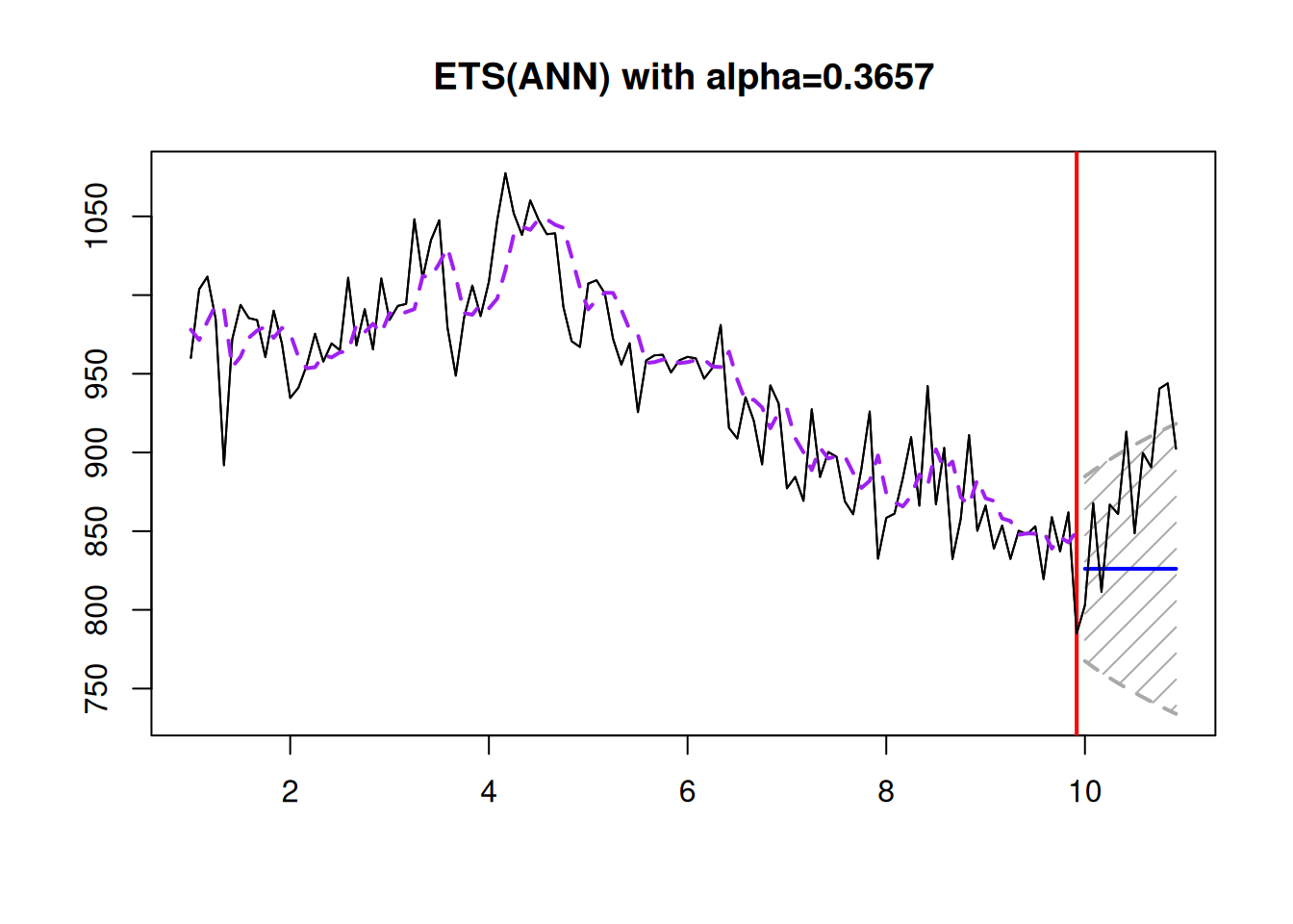
Figure 4.4: An example of ETS(A,N,N) applied to the data generated from the same model.
As we see from Figure 4.4, the true smoothing parameter is 0.3, but the estimated one is not exactly 0.3, which is expected because we deal with an in-sample estimation. Also, notice that with such a smoothing parameter, the prediction interval widens with the increase of the forecast horizon. If the smoothing parameter were lower, the bounds would not increase, but this might not reflect the uncertainty about the level correctly. Here is an example with \(\alpha=0.01\) on the same data (Figure 4.5).
es(y$data, "ANN", h=12,
   holdout=TRUE, persistence=0.01) |>
    forecast(h=12, interval="pred") |>
    plot(main="ETS(ANN) with alpha=0.01")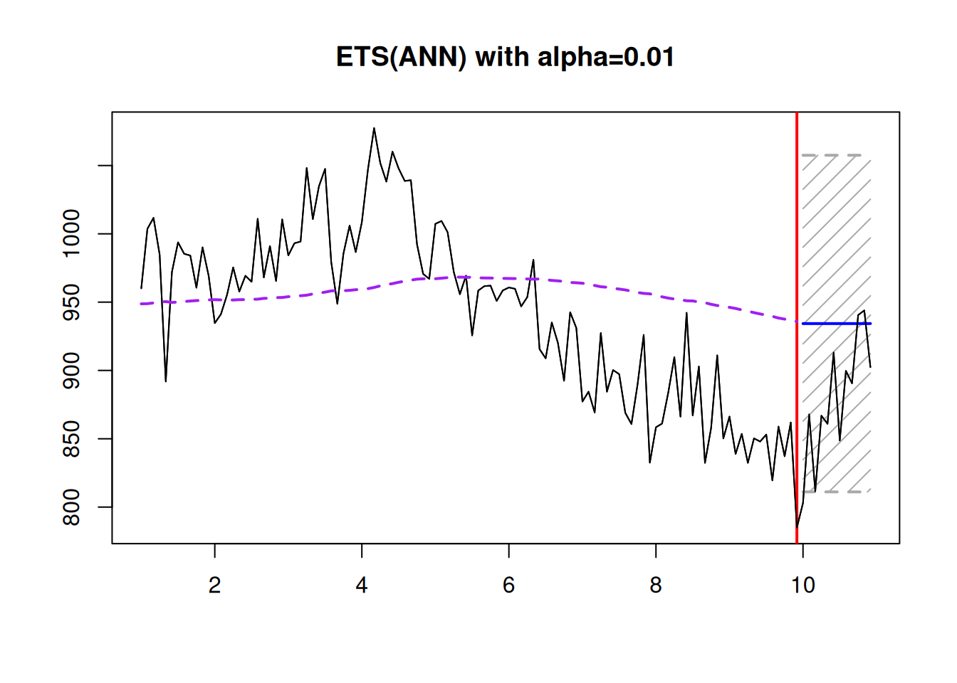
Figure 4.5: ETS(A,N,N) with \(\hat{\alpha}=0.01\) applied to the data generated from the same model with \(\alpha=0.3\).
Figure 4.5 shows that the prediction interval does not expand, but at the same time is wider than needed, and the forecast is biased – the model does not keep up to the fast-changing time series. So, it is essential to correctly estimate the smoothing parameters not only to approximate the data but also to produce a less biased point forecast and a more appropriate prediction interval.
4.3.2 ETS(M,N,N)
Hyndman et al. (2008) demonstrate that there is another ETS model, underlying SES. It is the model with multiplicative error, which is formulated in the following way, as mentioned in Chapter 4.2: \[\begin{equation} \begin{aligned} & y_{t} = l_{t-1}(1 + \epsilon_t) \\ & l_t = l_{t-1}(1 + \alpha \epsilon_t) \end{aligned} , \tag{4.6} \end{equation}\] where \((1+\epsilon_t)\) corresponds to the \(\varepsilon_t\) discussed in Section 3.1. If we open the brackets in the measurement equation of (4.6), we will see the main property of the ETS(M,N,N) - the variability in the model changes together with the level: \[\begin{equation} y_{t} = l_{t-1} + l_{t-1} \epsilon_t . \tag{4.7} \end{equation}\] So, if the error term had a standard deviation of 0.05, the standard deviation of the data would be \(l_{t-1} \times 0.05\). This means that the model captures the percentage deviation in the data rather than the unit one as in the ETS(A,N,N).
In order to see the connection of this model with SES, we need to revert to the estimation of the model on the data again: \[\begin{equation} \begin{aligned} & y_{t} = \hat{l}_{t-1}(1 + e_t) \\ & \hat{l}_t = \hat{l}_{t-1}(1 + \hat{\alpha} e_t) \end{aligned} . \tag{4.8} \end{equation}\] where the one step ahead forecast is (Section 4.2) \(\hat{y}_t = \hat{l}_{t-1}\) and \(e_t=\frac{y_t -\hat{y}_t}{\hat{y}_t}\). Substituting these values in the second equation of (4.8) we obtain: \[\begin{equation} \hat{y}_{t+1} = \hat{y}_t \left(1 + \hat{\alpha} \frac{y_t -\hat{y}_t}{\hat{y}_t} \right) \tag{4.9} \end{equation}\] Finally, opening the brackets, we get the SES in the form similar to (3.21): \[\begin{equation} \hat{y}_{t+1} = \hat{y}_t + \hat{\alpha} (y_t -\hat{y}_t). \tag{4.10} \end{equation}\]
This example again demonstrates the difference between a forecasting method and a model. When we use SES, we ignore the distributional assumptions, which restricts the usefulness of the method. When we work with a model, we assume a specific structure, which on the one hand, makes it more restrictive, but on the other hand, gives it additional features. The main ones in the case of ETS(M,N,N) in comparison with ETS(A,N,N) are:
- The variance of the actual values in ETS(M,N,N) increases with the increase of the level \(l_{t}\). This allows modelling a heteroscedasticity situation in the data;
- If \((1+\epsilon_t)\) is always positive, then the ETS(M,N,N) model will always produce only positive forecasts (both point and interval). This makes this model applicable in principle to the data with low levels.
An alternative to (4.6) would be the ETS(A,N,N) model (4.3) applied to the data in logarithms (assuming that the data we work with is always positive), implying that:
\[\begin{equation}
\begin{aligned}
& \log y_{t} = l_{t-1} + \epsilon_t \\
& l_t = l_{t-1} + \alpha \epsilon_t
\end{aligned} .
\tag{4.11}
\end{equation}\]
However, to produce forecasts from (4.11), exponentiation is needed, making the application of the model more difficult than needed. The ETS(M,N,N), on the other hand, does not rely on exponentiation, making it more practical and safe in cases when the model produces very high values (e.g. exp(1000) returns infinity in R).
Finally, the conditional \(h\) steps ahead mean of ETS(M,N,N) corresponds to the point forecast and is equal to the last observed level, but only if \(\mathrm{E}(1+\epsilon_t)=1\): \[\begin{equation} \mu_{y,t+h|t} = \hat{y}_{t+h} = l_{t} . \tag{4.12} \end{equation}\]
And here is an example with the ETS(M,N,N) data (Figure 4.6):
y <- sim.es("MNN", 120, 1, 12, persistence=0.3, initial=1000)
esModel <- es(y$data, "MNN", h=12, holdout=TRUE)
forecast(esModel, h=12, interval="pred") |>
    plot(main=paste0("ETS(MNN) with alpha=",
                     round(esModel$persistence,4)))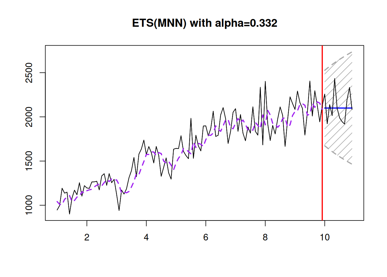
Figure 4.6: ETS(M,N,N) model applied to the data generated from the same model.
Conceptually, the data in Figure 4.6 looks very similar to the one from ETS(A,N,N) (Figure 4.4), but demonstrating the changing variance of the error term with the change of the level. The model itself would in general produce a wider prediction interval with the increase of the level than its additive error counterpart, keeping the same smoothing parameter.
4.3.3 ETS(A,N,N) vs ETS(M,N,N)
To better understand the difference between ETS(A,N,N) and ETS(M,N,N), consider the following example. I generated data from ETS(A,N,N) and ETS(M,N,N) using the sim.es() function from the smooth package with some predefined parameters to make the two comparable:
seed <- 50
set.seed(seed, kind="L'Ecuyer-CMRG")
y1 <- sim.es("ANN", 120, frequency=12,
             persistence=0.4, initial=500,
             mean=0, sd=25)
set.seed(seed, kind="L'Ecuyer-CMRG")
y2 <- sim.es("MNN", 120, frequency=12,
             persistence=0.4, initial=500,
             mean=1, sd=0.05)
Note that I fixed the random seed to have the same sequence of errors. I also set the standard deviations in the two models so that the error term variability in the beginning of the data is similar: \(l_{t-1} \times \epsilon_t = 500 \times 0.05 = 25\). In the ETS(A,N,N), the variability around the level will be on average around 25 units (based on the standard deviation used in the generation), while in the ETS(M,N,N), it should be around 5% (once again, based on the used DGP). Visually the generated data is shown in Figure 4.7.
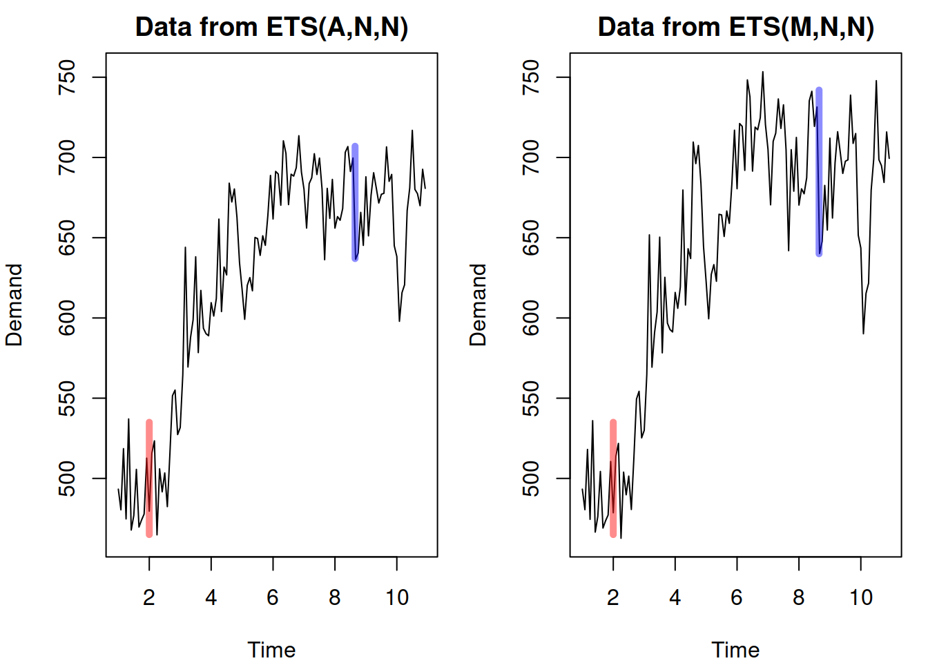
Figure 4.7: Data generated from ETS(A,N,N) and ETS(M,N,N).
The red lines in Figure 4.7 depict the initial variability in the data for the two time series, while the blue ones show the final one, when the level increased from 500 to roughly 700. As we see, the variability in the data generated using ETS(M,N,N) increased (to roughly \(700 \times 0.05 = 35\)), while in case of the ETS(A,N,N), it stayed the same (25). When we apply the ETS(A,N,N) and ETS(M,N,N) models to the respective data using the es() function from the smooth package, we get the model fit and forecasts shown in Figure 4.8.
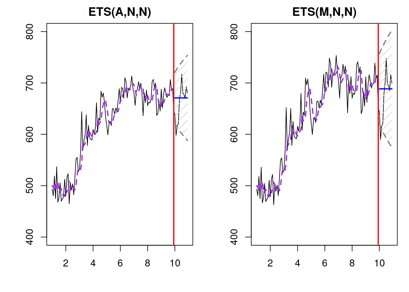
Figure 4.8: Data generated from ETS(A,N,N) and ETS(M,N,N).
Figure 4.8 demonstrates that although the two models produce very similar fit and point forecasts (because they had the same initial levels and smoothing parameters), the prediction interval in the ETS(M,N,N) is wider than in the ETS(A,N,N), reflecting the increased uncertainty due to the increase of the level.
Remark. The fact that the ETS(M,N,N) has the percentage variability rather than the unit one also means that if the level was to decrease, for example, to 200, the model would produce narrower prediction interval than the ETS(A,N,N) for the same values of the smoothing parameter. This follows directly from the formula for the error term in the model: \(l_{t-1} \times \epsilon_t = 200 \times 0.05 = 10\) vs the constant variability of 25 of the ETS(A,N,N).