14.5 Residuals are i.i.d.: Autocorrelation
One of the typical characteristics of time series models is the dynamic relation between variables. Even if fundamentally, the sales of ice cream on Monday do not impact sales of the same ice cream on Tuesday, they might impact sales of a competing product on Tuesday, Wednesday, or next week. Missing this structure might lead to the autocorrelation of residuals, influencing the estimates of parameters and final forecasts. This can influence the prediction intervals (causing miscalibration) and in serious cases can lead to biased forecasts. Autocorrelations might also arise due to wrong transformations of variables, where the model would systematically underforecast the actuals, producing autocorrelated residuals. In this section, we will see one of the potential ways for the diagnostics of this issue and try to improve the model in a stepwise manner, adding different orders of the ARIMA model (Section 9).
As an example, we continue with the same seatbelts data, dropping the dynamic part to see what would happen in this case:
adamSeat09 <- adam(Seatbelts, "NNN", lags=12,
                   formula=drivers~log(PetrolPrice)+log(kms)+law)
AICc(adamSeat09)
## [1] 2651.191There are different ways to diagnose the autocorrelation in this model. We start with a basic plot of residuals over time (Figure 14.16):
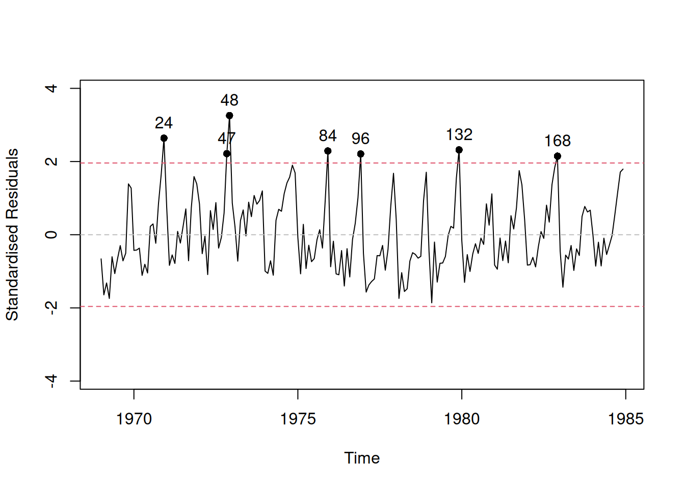
Figure 14.16: Standardised residuals vs time for Model 9.
We see in Figure 14.16 that on one hand the residuals still contain seasonality and on the other, they do not look stationary. We could conduct ADF and/or KPSS tests to get a formal answer to the stationarity question:
## Warning in tseries::kpss.test(resid(adamSeat09)): p-value greater than printed
## p-value
##
## KPSS Test for Level Stationarity
##
## data: resid(adamSeat09)
## KPSS Level = 0.12844, Truncation lag parameter = 4, p-value = 0.1## Warning in tseries::adf.test(resid(adamSeat09)): p-value smaller than printed
## p-value##
## Augmented Dickey-Fuller Test
##
## data: resid(adamSeat09)
## Dickey-Fuller = -6.8851, Lag order = 5, p-value = 0.01
## alternative hypothesis: stationaryThe tests have opposite null hypotheses, and in our case, we would fail to reject H\(_0\) on a 1% significance level for the KPSS test and reject H\(_0\) on the same level for the ADF, which means that the residuals look stationary. The main problem in the residuals is the seasonality, which formally makes the residuals non-stationary (their mean changes from month to month), but which cannot be detected by these tests. Yes, there is a Canova-Hansen test (implemented in the ch.test function of the uroot package in R), which tests the seasonal unit root, but instead of trying it out and coming to conclusions, I will try the model in seasonal differences and see if it is better than the one without it:
# SARIMAX(0,0,0)(0,1,0)_12
adamSeat10 <- adam(Seatbelts,"NNN",lags=12,
                   formula=drivers~log(PetrolPrice)+log(kms)+law,
                   orders=list(i=c(0,1)))
AICc(adamSeat10)
## [1] 2506.291Remark. While in general models in differences are not comparable with the models applied to the original data, adam() allows such comparison, because the ARIMA model implemented in it is initialised before the start of the sample and does not loose any observations.
This leads to an improvement in AICc in comparison with the previous model. The residuals of the model are now also better behaved (Figure 14.17):
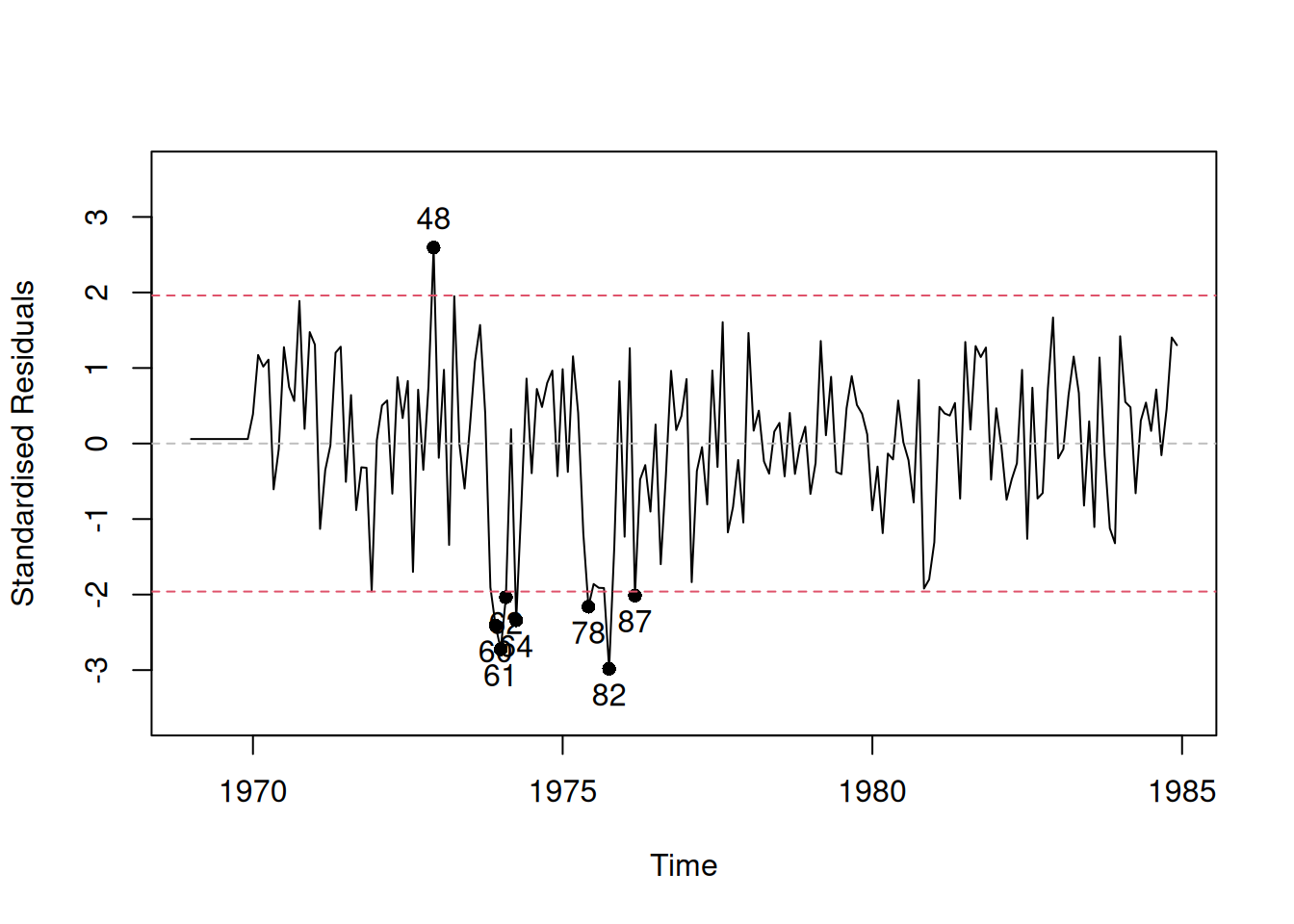
Figure 14.17: Standardised residuals vs time for Model 10.
In order to see whether there are any other dynamic elements left, we plot the ACF and PACF (discussed in Subsections 8.3.2 and 8.3.3) of residuals (Figure 14.18):
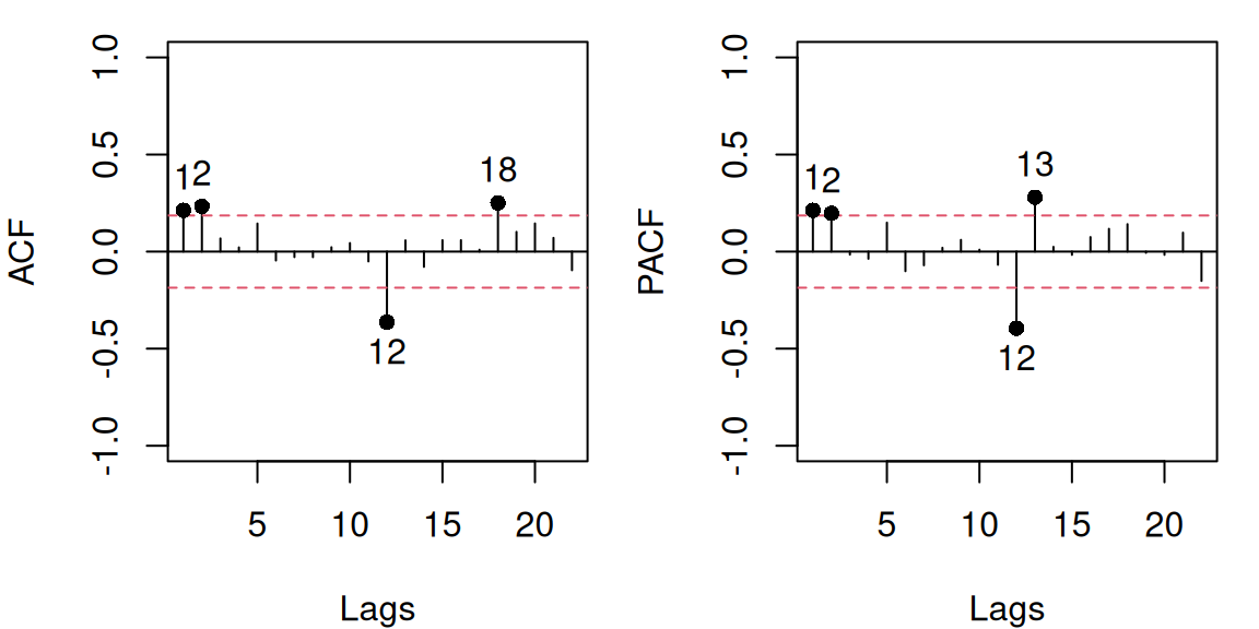
Figure 14.18: ACF and PACF of residuals of Model 10.
In the case of the adam objects, these plots, by default, will always have the range for the y-axis from -1 to 1 and will start from lag 1 on the x-axis. The red horizontal lines represent the “non-rejection” region. If a point lies inside the region, it is not statistically different from zero on the selected confidence level (the uncertainty around it is so high that it covers zero). The points with numbers are those that are statistically significantly different from zero. So, the ACF/PACF analysis might show the statistically significant lags on the selected level (the default one is 0.95, but I use level=0.99 in this section). Given that this is a statistical instrument, we expect that approximately (1-level)% (e.g. 1%) of lags will lie outside these bounds just due to randomness, even if the null hypothesis is correct. So it is okay if we do not see all points lying inside them. However, we should not see any patterns there, and we might need to investigate the suspicious lags to improve the model (low orders of up to 3 – 5 and the seasonal lags if they appear). In our example in Figure 14.18, we see that there are spikes in lag 12 for both ACF and PACF, which means that we have missed the seasonal element in the data. There is also a suspicious lag 1 on PACF and lags 1 and 2 on ACF, which could potentially indicate that MA(1) and/or AR(1), AR(2) elements are needed in the model. While it is not clear what specifically is needed here, we can try out several models and see which one is better to determine the appropriate order of ARIMA. We should start with the seasonal part of the model, as it is easier to deal with in the first step.
# SARIMAX(0,0,0)(1,1,0)_12
adamSeat11 <- adam(Seatbelts,"NNN",lags=12,
                   formula=drivers~log(PetrolPrice)+log(kms)+law,
                   orders=list(ar=c(0,1),i=c(0,1)))
AICc(adamSeat11)
## [1] 2474.548# SARIMAX(0,0,0)(0,1,1)_12
adamSeat12 <- adam(Seatbelts,"NNN",lags=12,
formula=drivers~log(PetrolPrice)+log(kms)+law,
orders=list(i=c(0,1),ma=c(0,1)))
AICc(adamSeat12)## [1] 2464.461# SARIMAX(0,0,0)(1,1,1)_12
adamSeat13 <- adam(Seatbelts,"NNN",lags=12,
formula=drivers~log(PetrolPrice)+log(kms)+law,
orders=list(ar=c(0,1),i=c(0,1),ma=c(0,1)))
AICc(adamSeat13)## [1] 2456.01Based on this analysis, we would be inclined to include the seasonal MA(1) only in the model. The next step in our iterative process – another ACF/PACF plot of the residuals to investigate whether there is anything else left:
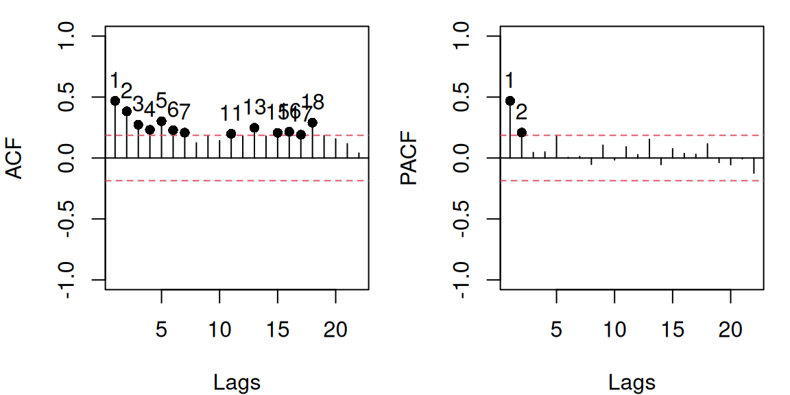
Figure 14.19: ACF and PACF of residuals of the model 12.
In this case, there is a spike on PACF for lag 1 and a textbook exponential decrease in ACF starting from lag 1, which might mean that we need to include AR(1) component in the model:
# ARIMAX(1,0,0)(0,1,1)_12
adamSeat14 <- adam(Seatbelts,"NNN",lags=12,
                   formula=drivers~log(PetrolPrice)+log(kms)+law,
                   orders=list(ar=c(1,0),i=c(0,1),ma=c(0,1)))
AICc(adamSeat14)
## [1] 2417.982Choosing between the new model and the old one, we should give preference to the former, which has a lower AICc than the previous one. So, adding AR(1) to the model leads to further improvement in AICc. Using this iterative procedure, we could continue our investigation to find the most suitable SARIMAX model for the data. We stop our discussion here, because this example should suffice in providing a general idea of how the diagnostics and the fix of autocorrelation issue can be done in ADAM. As an alternative, we could simplify the process and use the automated ARIMA selection algorithm (see discussion in Section 15.2). This is built on the principles discussed above (testing sequentially the potential orders based on ACF/PACF and AIC):
adamSeat15 <-
  adam(Seatbelts,"NNN",lags=12,
       formula=drivers~log(PetrolPrice)+log(kms)+law,
       orders=list(ar=c(3,2),i=c(2,1),ma=c(3,2),select=TRUE))
adamSeat15$model
## [1] "SARIMAX(0,1,1)[1](0,1,1)[12]"## [1] 2411.379This newly constructed model is SARIMAX(2,0,0)(0,1,1)\(_{12}\), which differs from the model that we achieved manually. Its residuals are better behaved than the ones of Model 5 (although we might need to analyse the residuals for the potential outliers, as discussed in Subsection 14.4):
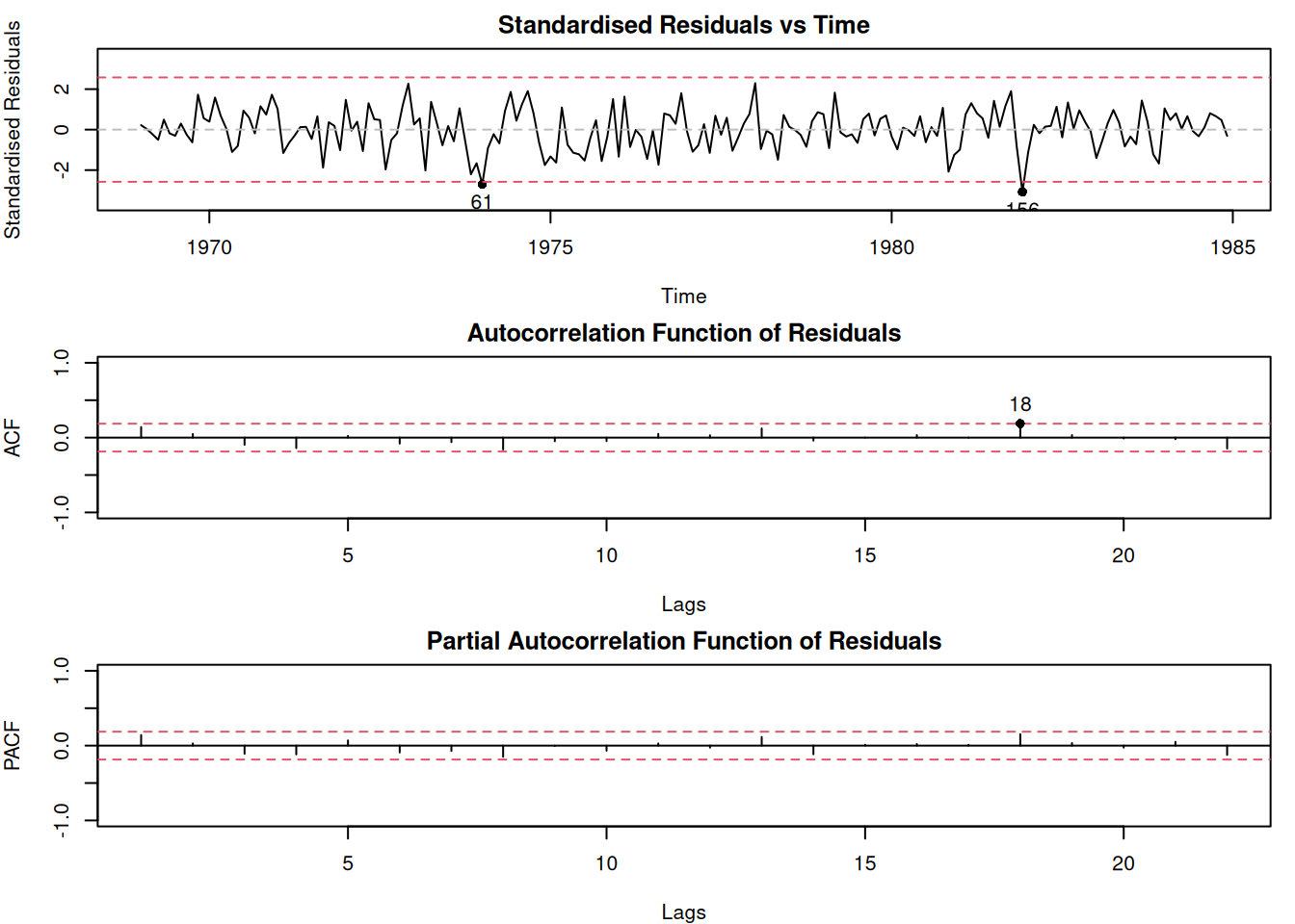
Figure 14.20: Residuals of Model 16.
As a final word for this section, we have focused our discussion on the visual analysis of time series, ignoring the statistical tests (we only used ADF and KPSS). Yes, there is the Durbin-Watson (Durbin and Watson, 1950) test for AR(1) in residuals, and yes, there are Ljung-Box (Ljung and Box, 1978), Box-Pierce (Box and Pierce, 1970) and Breusch-Godfrey (Breusch, 1978; Godfrey, 1978) tests for multiple AR elements. But visual inspection of time series is not less powerful than hypothesis testing. It makes you think and analyse the model and its assumptions, while the tests are the lazy way out that might lead to wrong conclusions because they have the standard limitations of any hypotheses tests (as discussed in Section 7.1 of Svetunkov and Yusupova, 2025). After all, if you fail to reject H\(_0\), it does not mean that the effect does not exist. Having said that, the statistical tests become extremely useful when you need to process many time series simultaneously and cannot inspect them manually. So, if you are in that situation, I would recommend reading more about them (even Wikipedia has good articles about them).
14.5.1 Correlations of multistep forecast errors
As a reminder, the multistep forecast errors are generated by producing 1 to \(h\) steps ahead forecasts from each observation in-sample starting from \(t=1\) and ending with \(t=T-h\) and subtracting it from the respective actual values. We have already discussed them and loss functions based on them in Section 11.3. They can be a useful diagnostic instrument, but they have one important property, which is sometimes ignored by researchers. In contrast with the residual \(e_t\), which is expected not to be autocorrelated, the forecast errors \(e_{t+i}\) and \(e_{t+j}\) for \(i \neq j\) should always be correlated if the persistence matrix of the model contains non-zero values. This is discussed by Svetunkov et al. (2023a) who showed that the only case when the forecast errors are uncorrelated is when the model is deterministic and does not have autocorrelated residuals. The correlation between the forecast errors will be stronger the closer \(i\) and \(j\) are to each other (e.g. it will be stronger between \(e_{t+3}\) and \(e_{t+4}\) than between \(e_{t+3}\) and \(e_{t+6}\)).
In R, the multistep forecast errors can be extracted via rmultistep() function from the smooth package. For demonstration purposes we use model 5:
# Extract multistep errors
adamSeat05ResidMulti <- rmultistep(adamSeat05, h=10)
# Give adequate names to the columns
colnames(adamSeat05ResidMulti) <- c(1:10)
# Calculate correlation matrix for forecast errors
cor(adamSeat05ResidMulti) |>
    round(3)
## 1 2 3 4 5 6 7 8 9 10
## 1 1.000 0.113 0.091 -0.025 -0.108 0.002 -0.086 -0.093 -0.197 -0.113
## 2 0.113 1.000 0.297 0.273 0.143 0.067 0.185 0.097 0.077 -0.030
## 3 0.091 0.297 1.000 0.341 0.304 0.172 0.114 0.212 0.125 0.094
## 4 -0.025 0.273 0.341 1.000 0.369 0.323 0.209 0.143 0.240 0.140
## 5 -0.108 0.143 0.304 0.369 1.000 0.376 0.339 0.211 0.148 0.231
## 6 0.002 0.067 0.172 0.323 0.376 1.000 0.383 0.332 0.204 0.127
## 7 -0.086 0.185 0.114 0.209 0.339 0.383 1.000 0.392 0.339 0.200
## 8 -0.093 0.097 0.212 0.143 0.211 0.332 0.392 1.000 0.399 0.334
## 9 -0.197 0.077 0.125 0.240 0.148 0.204 0.339 0.399 1.000 0.397
## 10 -0.113 -0.030 0.094 0.140 0.231 0.127 0.200 0.334 0.397 1.000As we can see from the output above, the correlations between the neighbouring forecast errors is higher than between the ones with larger distance. We cannot use this property for diagnostics purposes, it is just one of the features of dynamic models that we should keep in mind.