3.2 Multiple Linear Regression
While simple linear regression provides a basic understanding of the idea of capturing the relations between variables, it is obvious that in reality there are more than one external variable that would impact the response variable. This means that instead of (3.1) we should have: \[\begin{equation} y_t = a_0 + a_1 x_{1,t} + a_2 x_{2,t} + \dots + a_{k-1} x_{k-1,t} + \epsilon_t , \tag{3.7} \end{equation}\] where \(a_j\) is a \(j\)-th parameter for the respective \(j\)-th explanatory variable and there is \(k-1\) of them in the model, meaning that when we want to estimate this model, we will have \(k\) unknown parameters. The regression line of this model in population (aka expectation conditional on the values of explanatory variables) is: \[\begin{equation} \mu_{y,t} = \mathrm{E}(y_t | \mathbf{x}_t) = a_0 + a_1 x_{1,t} + a_2 x_{2,t} + \dots + a_{k-1} x_{k-1,t} , \tag{3.8} \end{equation}\] while in case of a sample estimation of the model we will use: \[\begin{equation} \hat{y}_t = \hat{a}_0 + \hat{a}_1 x_{1,t} + \hat{a}_2 x_{2,t} + \dots + \hat{a}_{k-1} x_{k-1,t} . \tag{3.9} \end{equation}\] While the simple linear regression can be represented as a line on the plane with an explanatory variable and a response variable, the multiple linear regression cannot be easily represented in the same way. In case of two explanatory variables the plot becomes three dimensional and the regression line transforms into regression plane.
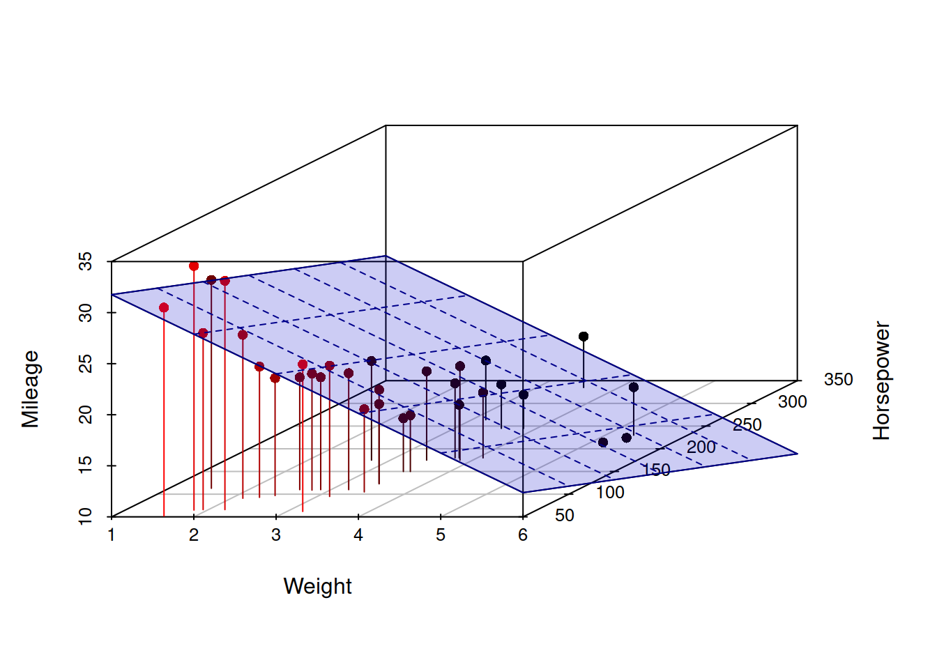
Figure 3.3: 3D scatterplot of Mileage vs Weight of a car and its Engine Horsepower.
Figure 3.3 demonstrates a three dimensional scatterplot with the regression plane, going through the points, similar to how the regression line went through the two dimensional scatterplot 3.1. These sorts of plots are already difficult to read, but the situation becomes even more challenging, when more than two explanatory variables are under consideration: plotting 4D, 5D etc is not a trivial task. Still, what can be said about the parameters of the model even if we cannot plot it in the same way, is that they represent slopes for each variable, in a similar manner as \(a_1\) did in the simple linear regression.
3.2.1 OLS estimation
In order to show how the estimation of multiple linear regression is done, we need to present it in a more compact form. In order to do that we will introduce the following vectors:
\[\begin{equation}
\mathbf{x}'_t = \begin{pmatrix}1 & x_{1,t} & \dots & x_{k-1,t} \end{pmatrix},
\boldsymbol{a} = \begin{pmatrix}a_0 \\ a_{1} \\ \vdots \\ a_{k-1} \end{pmatrix} ,
\tag{3.10}
\end{equation}\]
where \('\) symbol is the transposition. This can then be substituted in (3.7) to get:
\[\begin{equation}
y_t = \mathbf{x}'_t \boldsymbol{a} + \epsilon_t .
\tag{3.11}
\end{equation}\]
But this is not over yet, we can make it even more compact, if we pack all those values with index \(t\) in vectors and matrices:
\[\begin{equation}
\mathbf{X} = \begin{pmatrix} \mathbf{x}'_1 \\ \mathbf{x}'_2 \\ \vdots \\ \mathbf{x}'_T \end{pmatrix},
\mathbf{y} = \begin{pmatrix} y_1 \\ y_2 \\ \vdots \\ y_T \end{pmatrix},
\boldsymbol{\epsilon} = \begin{pmatrix} \epsilon_1 \\ \epsilon_2 \\ \vdots \\ \epsilon_T \end{pmatrix} ,
\tag{3.12}
\end{equation}\]
where \(T\) is the sample size. This leads to the following compact form of multiple linear regression:
\[\begin{equation}
\mathbf{y} = \mathbf{X} \boldsymbol{a} + \boldsymbol{\epsilon} .
\tag{3.13}
\end{equation}\]
Now that we have this compact form of multiple linear regression, we can estimate it using linear algebra. Many statistical textbooks explain how the following result is obtained (this involves taking derivative of SSE (3.4) with respect to \(\boldsymbol{a}\) and equating it to zero):
\[\begin{equation}
\hat{\boldsymbol{a}} = \left(\mathbf{X}' \mathbf{X}\right)^{-1} \mathbf{X}' \mathbf{y} .
\tag{3.14}
\end{equation}\]
The formula (3.14) is used in all the statistical software, including lm() function from stats package for R. Here is an example with the same mtcars dataset:
mtcarsModel01 <- lm(mpg~cyl+disp+hp++drat+wt+qsec+gear+carb, mtcars)The simplest plot that we can produce from this model is fitted values vs actuals, plotting \(\hat{y}_t\) on x-axis and \(y_t\) on the y-axis:
plot(fitted(mtcarsModel01),actuals(mtcarsModel01))
The same plot is produced via plot() method if we use alm() function from greybox instead:
mtcarsModel02 <- alm(mpg~cyl+disp+hp++drat+wt+qsec+gear+carb, mtcars, loss="MSE")
plot(mtcarsModel02,1)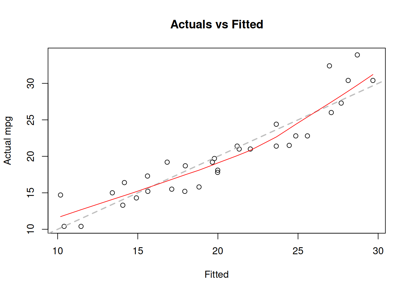
Figure 3.4: Actuals vs fitted values for multiple linear regression model on mtcars data.
We use loss="MSE" in this case, to make sure that the model is estimated via OLS. We will discuss the default estimation method in alm(), likelihood, in Section 3.7.
The plot on Figure 3.4 can be used for diagnostic purposes and in ideal situation the red line (LOWESS line) should coincide with the grey one, which would mean that we have correctly capture the tendencies in the data, so that all the regression assumptions are satisfied (see Section 3.6). We will come back to the model diagnostics in Section 17.
3.2.2 Quality of a fit
In order to get a general impression about the performance of the estimated model, we can calculate several in-sample measures, which could provide us insights about the fit of the model.
The first one is based on the OLS criterion, (3.4) and is called either “Root Mean Squared Error” (RMSE) or a “standard error” or a “standard deviation of error” of the regression: \[\begin{equation} \mathrm{RMSE} = \sqrt{\frac{1}{T-k} \sum_{t=1}^T e_t^2 }. \tag{3.15} \end{equation}\] Note that it is divided by the number of degrees of freedom in the model, \(T-k\), not on the number of observations. This is needed to correct the in-sample bias of the measure. RMSE does not tell us about the in-sample performance but can be used to compare several models with the same response variable between each other: the lower RMSE is, the better the model fits the data. Note that this measure is not aware of the randomness in the true model and thus will be equal to zero in a model that fits the data perfectly (thus ignoring the existence of error term). This is a potential issue, as we might end up with a poor model that would seem like the best one.
Here is how this can be calculated for our model, estimated using alm() function:
sigma(mtcarsModel02)## [1] 2.622011Another measure is called “Coefficient of Determination” and is calculated based on the following sums of squares: \[\begin{equation} \mathrm{R}^2 = 1 - \frac{\mathrm{SSE}}{\mathrm{SST}} = \frac{\mathrm{SSR}}{\mathrm{SST}}, \tag{3.16} \end{equation}\] where SSE$=_{t=1}^T e_t^2 $ is the OLS criterion defined in (3.4), \[\begin{equation} \mathrm{SST}=\sum_{t=1}^T (y_t - \bar{y})^2, \tag{3.17} \end{equation}\] is the total sum of squares (where \(\bar{y}\) is the in-sample mean) and \[\begin{equation} \mathrm{SSR}=\sum_{t=1}^T (\hat{y}_t - \bar{y})^2, \tag{3.18} \end{equation}\] is the sum of squares of the regression line. SSE, as discussed above, shows the overall distance of actual values from the regression line. The SST has an apparent connection with the variance of the response variable: \[\begin{equation} \mathrm{V}(y) = \frac{1}{T-1} \sum_{t=1}^T (y_t - \bar{y})^2 = \frac{1}{T-1} \mathrm{SST} . \tag{3.19} \end{equation}\] Finally, SSR characterises the deviation of the regression line from the mean. In the linear regression (this is important! This property might be violated in other models), the three sums are related via the following equation: \[\begin{equation} \mathrm{SST} = \mathrm{SSE} + \mathrm{SSR}, \tag{3.20} \end{equation}\] which explains why the coefficient of determination (3.16) can be calculated using two different formulae. If we want to interpret the coefficient of determination \(\mathrm{R}^2\), we can imagine the following situations:
- The model fits the data in the same way as a straight line (mean). In this case SSE would be equal to SST and SSR would be equal to zero (because \(\hat{y}_t=\bar{y}\)) and as a result the R\(^2\) would be equal to zero.
- The model fits the data perfectly, without any errors. In this situation SSE would be equal to zero and SSR would be equal to SST, because the regression would go through all points (i.e. \(\hat{y}_t=y_t\)). This would make R\(^2\) equal to one.
In the linear regression model due to (3.20), the coefficient of determination would always lie between zero and one, where zero means that the model does not explain the data at all and one means that it overfits the data. The value itself is usually interpreted as a percentage of variability in data explained by the model. This definition above provides us an important point about the coefficient of determination: it should not be equal to one, and it is alarming if it is very close to one - because in this situation we are implying that there is no randomness in the data, but this contradicts our definition of the statistical model (see Section 1.1). So, in practice we should not maximise R\(^2\) and should be careful with models that have very high values of it. At the same time, too low values of R\(^2\) are also alarming, as they tell us that the model is not very different from the global mean. So, coefficient of determination in general is not a very good measure for assessing performance of a model.
Here how this measure can be calculated in R based on the estimated model:
1 - sigma(mtcarsModel02)^2*(nobs(mtcarsModel02)-nparam(mtcarsModel02)) /
    (var(actuals(mtcarsModel02))*(nobs(mtcarsModel02)-1))
## [1] 0.8595764Note that in this formula we used the relation between SSE and RMSE and between SST and V\((y)\), multiplying the values by \(n-k\) and \(n-1\) respectively. The resulting value tells us that the model has explained 94.7% deviations in the data.
Based on coefficient of determination, we can also calculate the coefficient of multiple correlation, which we have already discussed in Section 2.6.4: \[\begin{equation} R = \sqrt{R^2} = \sqrt{\frac{\mathrm{SSR}}{\mathrm{SST}}} . \tag{3.21} \end{equation}\]
Furthermore, the value of coefficient of determination would always increase with the increase of number of variables included in the model. This is because every variable will explain some proportion of the data due to randomness. So, if we add redundant variables, the fit will improve, but the quality of model will decrease. Here is an example:
mtcarsData$noise <- rnorm(nrow(mtcarsData),0,10)
mtcarsModel02WithNoise <- alm(mpg~cyl+disp+hp++drat+wt+qsec+gear+carb+noise,
                                   mtcarsData, loss="MSE")
And here is the value of determination coefficient of the new model:
1 - sigma(mtcarsModel02WithNoise)^2*(nobs(mtcarsModel02WithNoise)-nparam(mtcarsModel02WithNoise)) /
    (var(actuals(mtcarsModel02WithNoise))*(nobs(mtcarsModel02WithNoise)-1))
## [1] 0.8639708The value in the new model will always be higher than in the previous one, no matter how we generate the random fluctuations. This means that some sort of penalisation of the number of variables in the model is required in order to make the measure more reasonable. This is what adjusted coefficient of determination is supposed to do: \[\begin{equation} R^2_{adj} = 1 - \frac{\mathrm{MSE}}{\mathrm{V}(y)} = 1 - \frac{(n-1)\mathrm{SSE}}{(n-k)\mathrm{SST}}, \tag{3.22} \end{equation}\] where MSE is the Mean Squared Error (square of RMSE (3.15)). So, instead of dividing sums of squares, in the adjusted R\(^2\) we divide the entities that are based on degrees of freedom. Given the presence of \(k\) in the formula (3.22), the coefficient will not necessarily increase with the addition of variables - when the variable does not contribute in the reduction of SSE of model substantially, R\(^2\) will not go up.
Here how it can be calculated for a model in R:
setNames(c(1 - sigma(mtcarsModel02)^2 / var(actuals(mtcarsModel02)),
           1 - sigma(mtcarsModel02WithNoise)^2 / var(actuals(mtcarsModel02WithNoise))),
         c("R^2-adj","R^2-adj, Noise"))
## R^2-adj R^2-adj, Noise
## 0.8107333 0.8083225What we hope to see in the output above is that the model with the noise will have a lower value of adjusted R\(^2\) than the model without it. However, given that we deal with randomness, if you reproduce this example many times, you will see different situation, including those, where introducing noise still increases the value of the parameter. So, you should not fully trust R\(^2_{adj}\) either. When constructing a model or deciding what to include in it, you should always use your judgement - make sure that the variables included in the model are meaningful. Otherwise you can easily overfit the data, which would lead to inaccurate forecasts and inefficient estimates of parameters (see Section 3.6 for details).
3.2.3 Interpretation of parameters
Finally, we come to the discussion of parameters of a model. As mentioned earlier, each one of them represents the slope of the model. But there is more to the meaning of parameters of the model. Consider the coefficients of the previously estimated model:
coef(mtcarsModel02)## (Intercept) cyl disp hp drat wt
## 17.88963741 -0.41459575 0.01293240 -0.02084886 1.10109551 -3.92064847
## qsec gear carb
## 0.54145693 1.23321026 -0.25509911Each of the parameters of this model shows an average effect of each variable on the mileage. They have a simple interpretation and show how the response variable will change on average with the increase of a variable by 1 unit, keeping all the other variables constant. For example, the parameter for wt (weight) shows that with the increase of weight of a car by 1000 pounds, the mileage would decrease on average by 3.921 miles per gallon, if all the other variables do not change. I have made the word “average” boldface three times in this paragraph for a reason. This is a very important point to keep in mind - the parameters will not tell you how variable will change for any specific observation. They do not show how it will change for each point. The regression model capture average tendencies and thus the word “average” is very important in the interpretation. In each specific case, the increase of weight by 1 will lead to different decreases (and even increases in some cases). But if we take the arithmetic mean of those individual effects, it will be close to the value of the parameter in the model. This however is only possible if all the assumptions of regression hold (see Section 3.6).