3.1 Simple Linear Regression
When we want to analyse some relations between variables, we can do graphical and correlations analysis. But this will not provide us sufficient information about what happens with the response variable with the change of explanatory variable. So it makes sense to consider the possible relations between variables, and the basis for this is Simple Linear Regression, which can be represented in the form: \[\begin{equation} y_t = a_0 + a_1 x_t + \epsilon_t , \tag{3.1} \end{equation}\] where \(a_0\) is the intercept (constant term), \(a_1\) is the coefficient for the slope parameter and \(\epsilon_t\) is the error term. The regression model is a basic statistical model that captures the relation between an explanatory variable \(x_t\) and the response variable \(y_t\). The parameters of the models are typically denoted as \(\beta_0\) and \(\beta_1\) in econometrics literature, but we use \(a_0\) and \(a_1\) because we will use \(\beta\) for other purposes later in this textbook.
In order to better understand what simple linear regression implies, consider the scatterplot (we discussed it earlier in Section 2.1.2) shown in Figure 3.1.
slmMPGWt <- lm(mpg~wt,mtcarsData)
plot(mtcarsData$wt, mtcarsData$mpg,
     xlab="Weight", ylab="Mileage",
     xlim=c(0,6), ylim=c(0,40))
abline(h=0, col="grey")
abline(v=0, col="grey")
abline(slmMPGWt,col="red")
text(4,35,paste0(c("mpg=",round(coef(slmMPGWt),2),"wt+et"),collapse=""))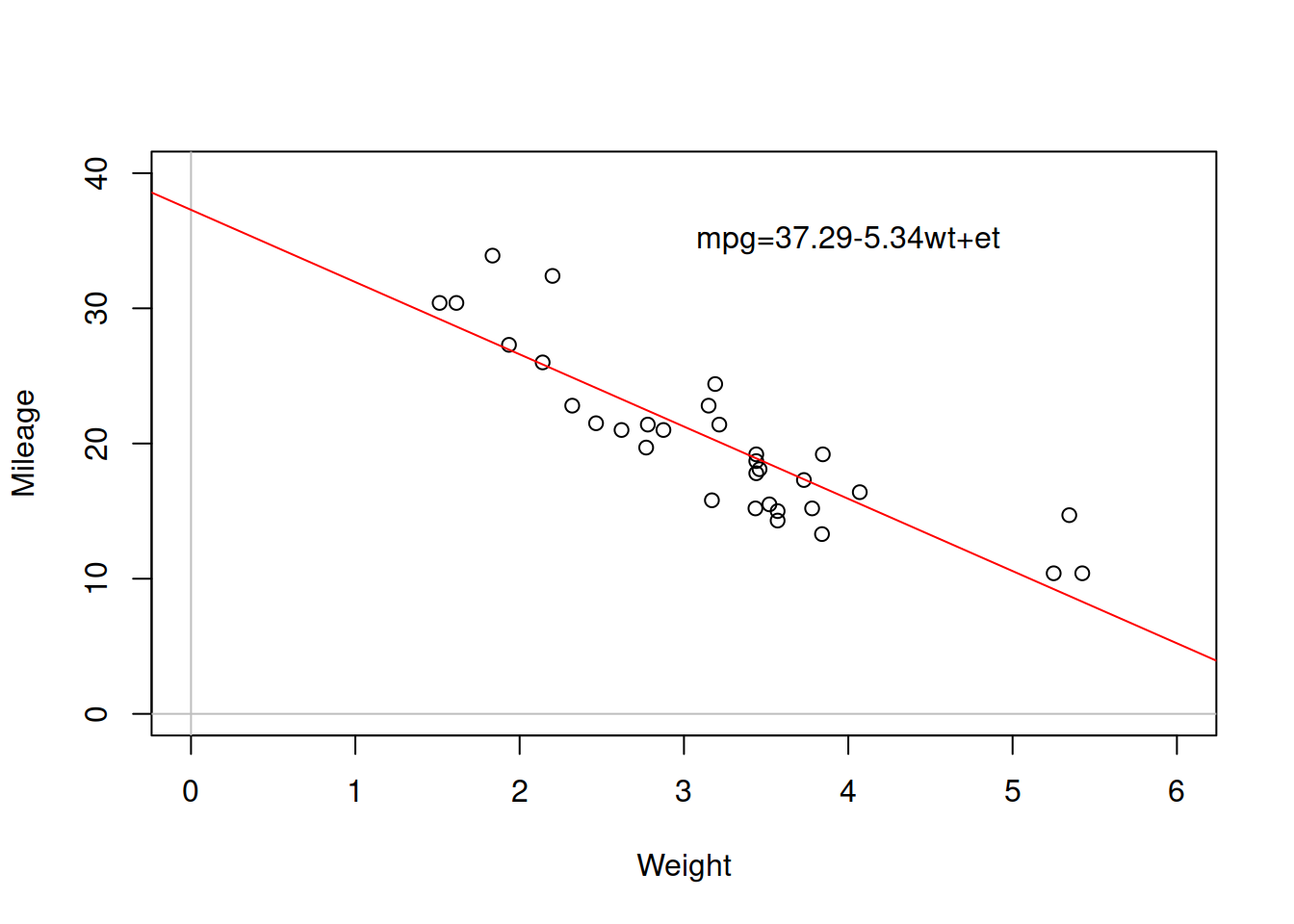
Figure 3.1: Scatterplot diagram between weight and mileage.
The line drawn on the plot is the regression line, parameters of which were estimated based on the available data. In this case the intercept \(\hat{a}_0\)=37.29, meaning that this is where the red line crosses the y-axis, while the parameter of slope \(\hat{a}_1\)=-5.34 shows how fast the values change (how steep the line is). I’ve added hat symbols on the parameters to point out that they were estimated based on a sample of data. If we had all the data in the universe (population) and estimated a correct model on it, we would not need the hats. In simple linear regression, the re line will always go through the cloud of points, showing the averaged out tendencies. The one that we observe above can be summarise as “with the increase of weight, on average the mileage of cars goes down.” Note that we might find some specific points, where the increase of weight would not decrease mileage (e.g. the two furthest left points show this), but this can be considered as a random fluctuation, so overall, the average tendency is as described above.
3.1.1 Ordinary Least Squares (OLS)
For obvious reasons, we do not have the values of parameters from the population. This means that we will never know what the true intercept and slope are. Luckily, we can estimate them based on the sample of data. There are different ways of doing that, and the most popular one is called “Ordinary Least Squares” method. This is the method that was used in the estimation of the model in Figure 3.1. So, how does it work?
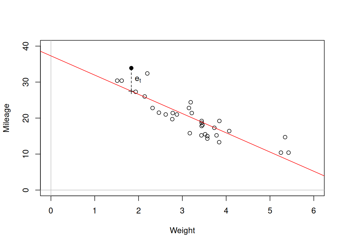
Figure 3.2: Scatterplot diagram between weight and mileage.
When we estimate the simple linear regression model, the model (3.1) transforms into: \[\begin{equation} y_t = \hat{a}_0 + \hat{a}_1 x_t + e_t . \tag{3.2} \end{equation}\] This is because we do not know the true values of parameters and thus they are substituted by their estimates. This also applies to the error term for which in general \(e_t \neq \epsilon_t\) because of the sample estimation. Now consider the same situation with weight vs mileage in Figure 3.2 but with some arbitrary line with unknown parameters. Each point on the plot will typically lie above or below the line, and we would be able to calculate the distances from those points to the line. They would correspond to \(e_t = y_t - \hat{y}_t\), where \(\hat{y}_t\) is the value of the regression line (aka “fitted” value) for each specific value of explanatory variable. For example, for the weight of car of 1.835 tones, the actual mileage is 33.9, while the fitted value is 27.478. The resulting error (or residual of model) is 6.422. We could collect all these errors of the model for all available cars based on their weights and this would result in a vector of positive and negative values like this:
##           Mazda RX4       Mazda RX4 Wag          Datsun 710      Hornet 4 Drive
##          -2.2826106          -0.9197704          -2.0859521           1.2973499
##   Hornet Sportabout             Valiant          Duster 360           Merc 240D
##          -0.2001440          -0.6932545          -3.9053627           4.1637381
##            Merc 230            Merc 280           Merc 280C          Merc 450SE
##           2.3499593           0.2998560          -1.1001440           0.8668731
##          Merc 450SL         Merc 450SLC  Cadillac Fleetwood Lincoln Continental
##          -0.0502472          -1.8830236           1.1733496           2.1032876
##   Chrysler Imperial            Fiat 128         Honda Civic      Toyota Corolla
##           5.9810744           6.8727113           1.7461954           6.4219792
##       Toyota Corona    Dodge Challenger         AMC Javelin          Camaro Z28
##          -2.6110037          -2.9725862          -3.7268663          -3.4623553
##    Pontiac Firebird           Fiat X1-9       Porsche 914-2        Lotus Europa
##           2.4643670           0.3564263           0.1520430           1.2010593
##      Ford Pantera L        Ferrari Dino       Maserati Bora          Volvo 142E
##          -4.5431513          -2.7809399          -3.2053627          -1.0274952
This corresponds to the formula: \[\begin{equation} e_t = y_t - \hat{a}_0 - \hat{a}_1 x_t. \tag{3.3} \end{equation}\] If we needed to estimate parameters \(\hat{a}_0\) and \(\hat{a}_1\) of the model, we would need to minimise those distances by changing the parameters of the model. The problem is that some errors are positive, while the others are negative. If we just sum them up, they will cancel each other out, and we would loose the information about the distance. The simplest way to get rid of sign and keep the distance is by taking squares of each error and calculating Sum of Squared Errors for the whole sample \(T\): \[\begin{equation} \mathrm{SSE} = \sum_{t=1}^T e_t^2 . \tag{3.4} \end{equation}\] If we now minimise SSE by changing values of parameters \(\hat{a}_0\) and \(\hat{a}_1\), we will find those parameters that would guarantee that the line goes somehow through the cloud of points. Luckily, we do not need to use any fancy optimisers for this, as this has analytical solution (in order to get it, insert (3.3) in (3.4), take derivatives with respect to the parameters \(\hat{a}_0\) and \(\hat{a}_1\) and equate the resulting values to zero): \[\begin{equation} \begin{aligned} \hat{a}_1 = & \frac{\mathrm{cov}(x,y)}{\mathrm{V}(x)} \\ \hat{a}_0 = & \bar{y} - \hat{a}_1 \bar{x} \end{aligned} , \tag{3.5} \end{equation}\] where \(\bar{x}\) is the mean of the explanatory variable \(x_t\) and \(\bar{y}\) is the mean of the response variables \(y_t\). Note that if for some reason \(\hat{a}_1=0\) (for example, because the covariance between \(x\) and \(y\) is zero, implying that they are not correlated), then the intercept \(\hat{a}_0 = \bar{y}\), meaning that the global average of the data is the best predictor of the variable \(y_t\). This method of estimation of parameters based on the minimisation of SSE, is called “Ordinary Least Squares.” It is simple and does not require any specific assumptions: we just minimise the overall distance by changing the values of parameters.
Another thing to note is the connection between the parameter \(\hat{a}_1\) and the correlation coefficient. We have already briefly discussed this in Section 2.6.3, we could estimate two models given the pair of variable \(x\) and \(y\):
- Model (3.2);
- The inverse model \(x_t = \hat{b}_0 + \hat{b}_1 y_t + u_t\).
We could then extract the slope parameters of the two models via (3.5) and get the value of correlation coefficient as a geometric mean of the two: \[\begin{equation} r_{x,y} = \mathrm{sign}(\hat{b}_1) \sqrt{\hat{a}_1 \hat{b}_1} = \mathrm{sign}(\mathrm{cov}(x,y)) \sqrt{\frac{\mathrm{cov}(x,y)}{\mathrm{V}(x)} \frac{\mathrm{cov}(x,y)}{\mathrm{V}(y)}} = \frac{\mathrm{cov}(x,y)}{\sqrt{V(x)V(y)}} , \tag{3.6} \end{equation}\] which is the formula (2.15). This is how the correlation coefficient was originally derived.
While we can do some inference based on simple linear regression, we know that the bivariate relations are not often met in practice: typically a variable is influenced by a set of variables, not just by one. This implies that the correct model would typically include many explanatory variables. This is why we will discuss inference in the next section.