3.3 Regression uncertainty
Coming back to the example of mileage vs weight of cars, the estimated simple linear regression on the data was mpg=37.29-5.34wt+et. But what would happen if we estimate the same model on a different sample of data (e.g. 15 first observations instead of 32)?
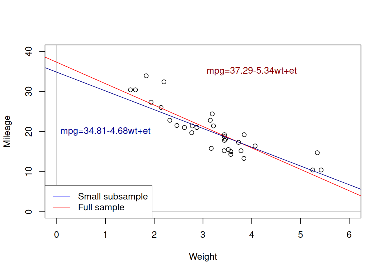
Figure 3.5: Weight vs mileage and two regression lines.
Figure 3.5 shows the two lines: the red one corresponds to the larger sample, while the blue one corresponds to the small one. We can see that these lines have different intercepts and slope parameters. So, which one of them is correct? An amateur analyst would say that the one that has more observations is the correct model. But a more experienced statistician would tell you that none of the two is correct. They are both estimated on a sample of data and they both inevitably inherit the uncertainty of the data, making them both incorrect if we compare them to the hypothetical true model. This means that whatever regression model we estimate on a sample of data, it will be incorrect as well.
This uncertainty about the regression line actually comes to the uncertainty of estimates of parameters of the model. In order to see it more clearly, consider the example with Speed and Stopping Distances of Cars dataset from datasets package (?cars):
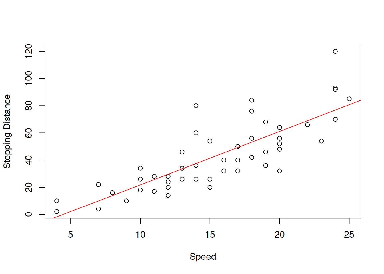
Figure 3.6: Speed vs stopping distance of cars
While the linear relation between these variables might be not the the most appropriate, it suffices for demonstration purposes. What we will do for this example is fit the model and then use a simple bootstrap technique to get estimates of parameters of the model. We will do that using coefbootstrap() method from greybox package. The bootstrap technique implemented in the function applies the same model to subsamples of the original data and returns a matrix with parameters. This way we get an idea about the empirical uncertainty of parameters:
slmSpeedDistanceBootstrap <- coefbootstrap(slmSpeedDistance)Based on that we can plot the histograms of the estimates of parameters.
par(mfcol=c(1,2))
hist(slmSpeedDistanceBootstrap$coefficients[,1],
     xlab="Intercept", main="")
hist(slmSpeedDistanceBootstrap$coefficients[,2],
     xlab="Slope", main="")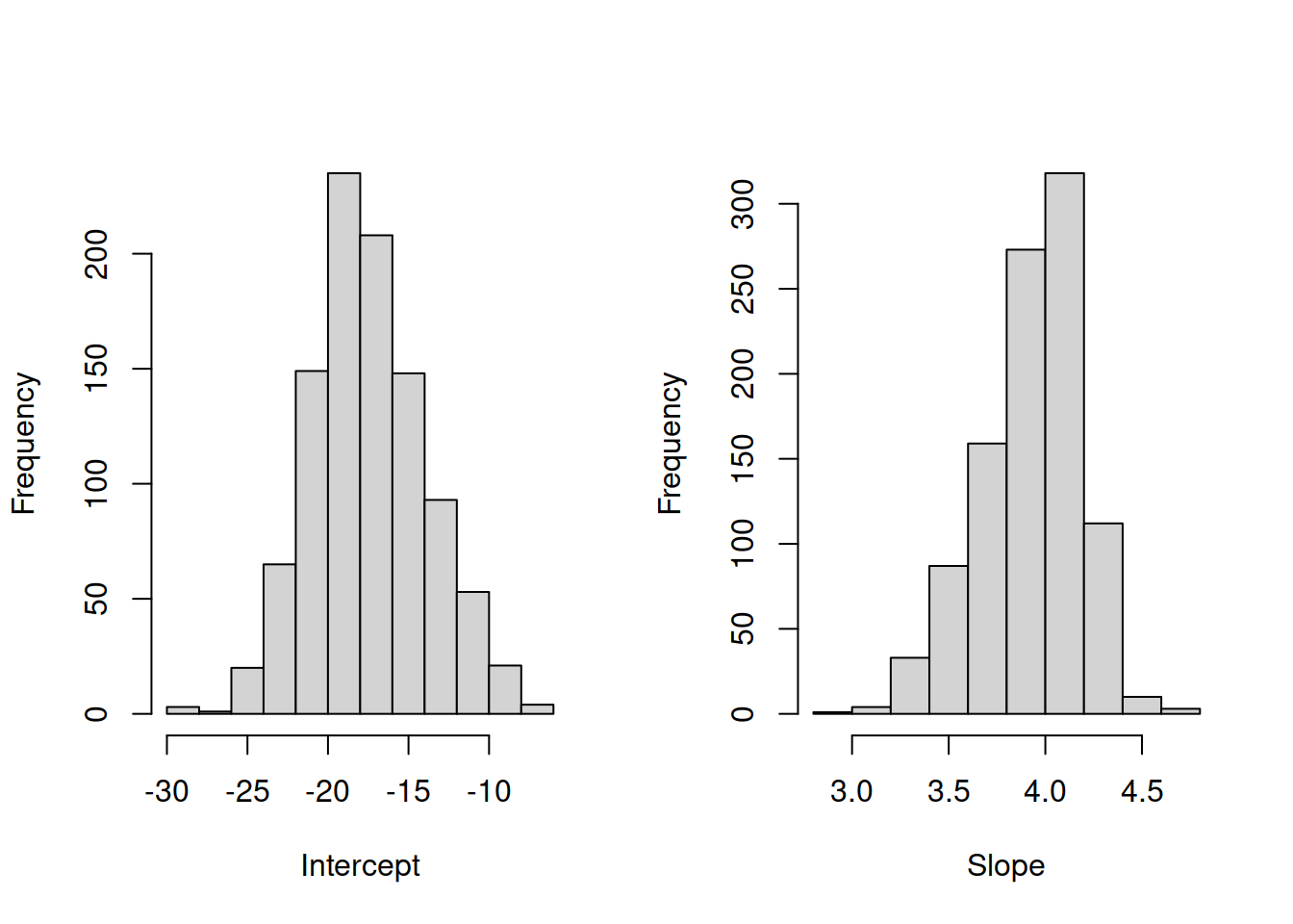
Figure 3.7: Distribution of bootstrapped parameters of a regression model
Figure 3.7 shows the uncertainty around the estimates of parameters. These distributions look similar to the normal distribution. In fact, if we repeated this example thousands of times, the distribution of estimates of parameters would indeed follow the normal one due to CLT (if the assumptions hold, see Sections 2.2.2 and 3.6). As a result, when we work with regression we should take this uncertainty about the parameters into account. This applies to both parameters analysis and forecasting.
3.3.1 Confidence intervals
In order to take this uncertainty into account, we could construct confidence intervals for the estimates of parameters, using the principles discussed in Section 2.4. This way we would hopefully have some idea about the uncertainty of the parameters, and not just rely on average values. If we assume that CLT holds, we could use the t statistics for the calculation of the quantiles of distribution (we need to use t because we do not know the variance of estimates of parameters). But in order to do that, we need to have variances of estimates of parameters. One of possible ways of getting them would be the bootstrap used in the example above. However, this is a computationally expensive operation, and there is a more efficient procedure, which however only works with linear regression models either estimated using OLS or via Maximum Likelihood Estimation assuming Normal distribution (see Section 3.7). In these conditions the covariance matrix of parameters can be calculated using the following formula: \[\begin{equation} \mathrm{V}(\hat{\mathbf{a}}) = \frac{1}{T-k} \sum_{t=1}^T e_t^2 \times \left(\mathbf{X}' \mathbf{X}\right)^{-1}. \tag{3.23} \end{equation}\] This matrix will contain variances of parameters on the diagonal and covariances between the parameters on off-diagonals. In this specific case, we only need the diagonal elements. We can take square root of them to obtain standard errors of parameters, which can then be used to construct confidence intervals for each parameter \(j\) via: \[\begin{equation} a_j \in (\hat{a}_j + t_{\alpha/2}(T-k) s_{\hat{a}_j}, \hat{a}_j + t_{1-\alpha/2}(T-k) s_{\hat{a}_j}), \tag{3.23} \end{equation}\] where \(s_{\hat{a}_j}\) is the standard error of the parameter \(\hat{a}_j\). All modern software does all these calculations automatically, so we do not need to do them manually. Here is an example:
vcov(slmSpeedDistance)## (Intercept) speed
## (Intercept) 45.676514 -2.6588234
## speed -2.658823 0.1726509This is the covariance matrix of parameters, the diagonal elements of which are then used in the confint() method:
confint(slmSpeedDistance)## S.E. 2.5% 97.5%
## (Intercept) 6.7584402 -31.167850 -3.990340
## speed 0.4155128 3.096964 4.767853The confidence interval for speed above shows, for example, that if we repeat the construction of interval many times, the true value of parameter speed will lie in 95% of cases between 3.08 and 4.78. This gives an idea about the real effect in the population. We can also present all of this in the following summary (this is based on the alm() model, the other functions will produce different summaries):
summary(slmSpeedDistance)## Response variable: dist
## Distribution used in the estimation: Normal
## Loss function used in estimation: MSE
## Coefficients:
## Estimate Std. Error Lower 2.5% Upper 97.5%
## (Intercept) -17.5791 6.7584 -31.1678 -3.9903 *
## speed 3.9324 0.4155 3.0970 4.7679 *
##
## Error standard deviation: 15.3796
## Sample size: 50
## Number of estimated parameters: 2
## Number of degrees of freedom: 48
## Information criteria:
## AIC AICc BIC BICc
## 417.1569 417.4122 420.9809 421.4803This summary provide all the necessary information about the estimates of parameters: their mean values in the column “Estimate,” their standard errors in “Std. Error,” the bounds of confidence interval and finally a star if the interval does not contain zero. This typically indicates that we are certain on the selected confidence level (95% in our example) about the sign of the parameter and that the effect really exists.
3.3.2 Hypothesis testing
Another way to look at the uncertainty of parameters is to test a statistical hypothesis. As it was discussed in Section 2.5, I personally think that hypothesis testing is a less useful instrument for these purposes than the confidence interval and that it might be misleading in some circumstances. Nonetheless, it has its merits and can be helpful if an analyst knows what they are doing. In order to test the hypothesis, we need to follow the procedure, described in Section 2.5.
The classical hypotheses for the parameters are formulated in the following way: \[\begin{equation} \begin{aligned} \mathrm{H}_0: a_j = 0 \\ \mathrm{H}_1: a_j \neq 0 \end{aligned} . \tag{3.24} \end{equation}\] This formulation of hypotheses comes from the idea that we want to check if the effect estimated by the regression is indeed there (i.e. statistically significantly different from zero). Note however, that as in any other hypothesis testing, if you fail to reject the null hypothesis, this only means that you do not know, we do not have enough evidence to conclude anything. This does not mean that there is no effect and that the respective variable can be removed from the model. In case of simple linear regression, the null and alternative hypothesis can be represented graphically as shown in Figure 3.8.
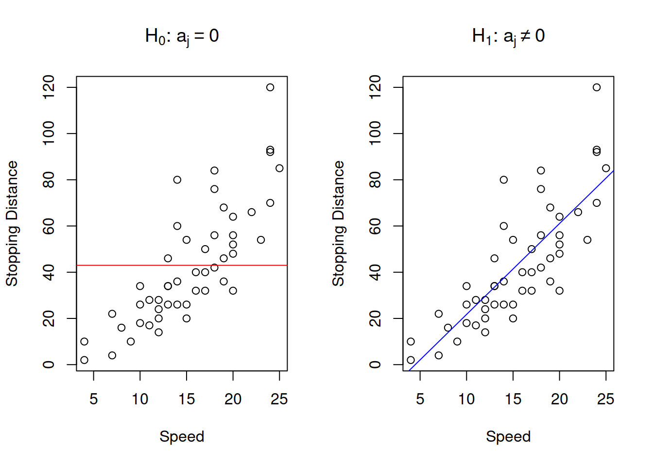
Figure 3.8: Graphical presentation of null and alternative hypothesis in regression context
The graph on the left in Figure 3.8 demonstrates how the true model could look if the null hypothesis was true - it would be just a straight line, parallel to x-axis. The graph on the right demonstrates the alternative situation, when the parameter is not equal to zero. We do not know the true model, and hypothesis testing does not tell us, whether the hypothesis is true or false, but if we have enough evidence to reject H\(_0\), then we might conclude that we see an effect of one variable on another in the data. Note, as discussed in Section 2.5, the null hypothesis is always wrong, and it will inevitably be rejected with the increase of sample size.
Given the discussion in the previous subsection, we know that the parameters of regression model will follow normal distribution, as long as all assumptions are satisfied (including those for CLT). We also know that because the standard errors of parameters are estimated, we need to use Student’s distribution, which takes the uncertainty about the variance into account. Based on this, we can say that the following statistics will follow t with \(T-k\) degrees of freedom: \[\begin{equation} \frac{\hat{a}_j - 0}{s_{\hat{a}_j}} \sim t(T-k) . \tag{3.25} \end{equation}\] After calculating the value and comparing it with the critical t-value on the selected significance level or directly comparing p-value based on (3.25) with the significance level, we can make conclusions about the hypothesis.
The context of regression provides a great example, why we never accept hypothesis and why in the case of “Fail to reject H\(_0\),” we should not remove a variable (unless we have more fundamental reasons for doing that). Consider an example, where the estimated parameter \(\hat{a}_1=0.5\), and its standard error is \(s_{\hat{a}_1}=1\), we estimated a simple linear regression on a sample of 30 observations, and we want to test, whether the parameter in the population is zero (i.e. hypothesis (3.24)) on 1% significance level. Inserting the values in formula (3.25), we get: \[\begin{equation*} \frac{|0.5 - 0|}{1} = 0.5, \end{equation*}\] with the critical value for two-tailed test of \(t_{0.01}(30-2)\approx 2.76\). Comparing t-value with the critical one, we would conclude that we fail to reject H\(_0\) and thus the parameter is not statistically different from zero. But what would happen if we check another hypothesis: \[\begin{equation*} \begin{aligned} \mathrm{H}_0: a_1 = 1 \\ \mathrm{H}_1: a_1 \neq 1 \end{aligned} . \end{equation*}\] The procedure is the same, the calculated t-value is: \[\begin{equation*} \frac{|0.5 - 1|}{1} = 0.5, \end{equation*}\] which leads to exactly the same conclusion as before: on 1% significance level, we fail to reject the new H\(_0\), so the value is not distinguishable from 1. So, which of the two is correct? The correct answer is “we do not know.” The non-rejection region just tells us that uncertainty about the parameter is so high that it also include the value of interest (0 in case of the classical regression analysis). If we constructed the confidence interval for this problem, we would not have such confusion, as we would conclude that on 1% significance level the true parameter lies in the region \((-2.26, 3.26)\) and can be any of these numbers.
In R, if you want to test the hypothesis for parameters, I would recommend using lm() function for regression:
lmSpeedDistance <- lm(dist~speed,cars)
summary(lmSpeedDistance)
##
## Call:
## lm(formula = dist ~ speed, data = cars)
##
## Residuals:
## Min 1Q Median 3Q Max
## -29.069 -9.525 -2.272 9.215 43.201
##
## Coefficients:
## Estimate Std. Error t value Pr(>|t|)
## (Intercept) -17.5791 6.7584 -2.601 0.0123 *
## speed 3.9324 0.4155 9.464 1.49e-12 ***
## ---
## Signif. codes: 0 '***' 0.001 '**' 0.01 '*' 0.05 '.' 0.1 ' ' 1
##
## Residual standard error: 15.38 on 48 degrees of freedom
## Multiple R-squared: 0.6511, Adjusted R-squared: 0.6438
## F-statistic: 89.57 on 1 and 48 DF, p-value: 1.49e-12This output tells us that when we consider the parameter for the variable speed, we reject the standard H\(_0\) on the pre-selected 1% significance level (comparing the level with p-value in the last column of the output). Note that we should first select the significance level and only then conduct the test, otherwise we would be bending reality for our needs.
Finally, in regression context, we can test another hypothesis, which becomes useful, when a lot of parameters of the model are very close to zero and seem to be insignificant on the selected level:
\[\begin{equation}
\begin{aligned}
\mathrm{H}_0: a_1 = a_2 = \dots = a_{k-1} = 0 \\
\mathrm{H}_1: a_1 \neq 0 \vee a_2 \neq 0 \vee \dots \vee a_{k-1} \neq 0
\end{aligned} ,
\tag{3.26}
\end{equation}\]
which translates into normal language as “H\(_0\): all parameters (except for intercept) are equal to zero; H\(_1\): at least one parameter is not equal to zero.” This is tested based on F statistics with \(k-1\), \(T-k\) degrees of freedom and is reported, for example, by lm() (see the last line in the previous output). This hypothesis is not very useful, when the parameter are significant and coefficient of determination is high. It only becomes useful in difficult situations of poor fit. The test on its own does not tell if the model is adequate or not. And the F value and related p-value is not comparable with respective values of other models. Graphically, this test checks, whether in the true model the slope of the straight line on the plot of actuals vs fitted is different from zero. An example with the same stopping distance model is provided in Figure 3.9.
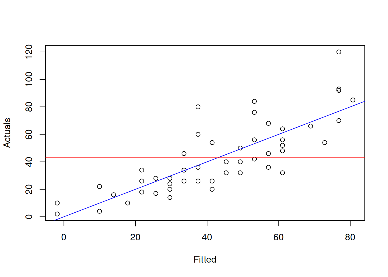
Figure 3.9: Graphical presentation of F test for regression model.
What the test is tries to get insight about, is whether in the true model the blue line coincides with the red line (i.e. the slope is equal to zero, which is only possible, when all parameters are zero). If we have enough evidence to reject the null hypothesis, then this means that the slopes are different on the selected significance level.
3.3.3 Regression model uncertainty
Given the uncertainty of estimates of parameters, the regression line itself and the points around it will be uncertain. This means that in some cases we should not just consider the predicted values of the regression \(\hat{y}_t\), but also the uncertainty around them.
The uncertainty of the regression line builds upon the uncertainty of parameters and can be measured via the conditional variance in the following way: \[\begin{equation} \mathrm{V}(\hat{y}_t| \mathbf{x}_t) = \mathrm{V}(\hat{a}_0 + \hat{a}_1 x_{1,t} + \hat{a}_2 x_{2,t} + \dots + \hat{a}_{k-1} x_{k-1,t}) , \tag{3.27} \end{equation}\] which after some simplifications leads to: \[\begin{equation} \mathrm{V}(\hat{y}_t| \mathbf{x}_t) = \sum_{j=0}^{k-1} \mathrm{V}(\hat{a}_j) x^2_{j,t} + 2 \sum_{j=1}^{k-1} \sum_{i=0}^{j-1} \mathrm{cov}(\hat{a}_i,\hat{a}_j) x_{i,t} x_{j,t} , \tag{3.28} \end{equation}\] where \(x_{0,t}=1\). As we see, the variance of the regression line involves variances and covariances of parameters. This variance can then be used in the construction of the confidence interval for the regression line. Given that each estimate of parameter \(\hat{a}_j\) will follow normal distribution with a fixed mean and variance due to CLT, the predicted value \(\hat{y}_t\) will follow normal distribution as well. This can be used in the construction of the confidence interval, in a manner similar to the one discussed in Section 2.4: \[\begin{equation} \mu \in (\hat{y}_t + t_{\alpha/2}(T-k) s_{\hat{y}_t}, \hat{y}_t + t_{1-\alpha/2}(T-k) s_{\hat{y}_t}), \tag{3.29} \end{equation}\] where \(s_{\hat{y}_t}=\sqrt{\mathrm{V}(\hat{y}_t| \mathbf{x}_t)}\).
In R, this interval can be constructed via the function predict() with interval="confidence". It is based on the covariance matrix of parameters, extracted via vcov() method in R (it was discussed in a previous subsection). Note that the interval can be produced not only for the in-sample value, but for the holdout as well. Here is an example with alm() function:
slmSpeedDistanceCI <- predict(slmSpeedDistance,interval="confidence")
plot(slmSpeedDistanceCI, main="")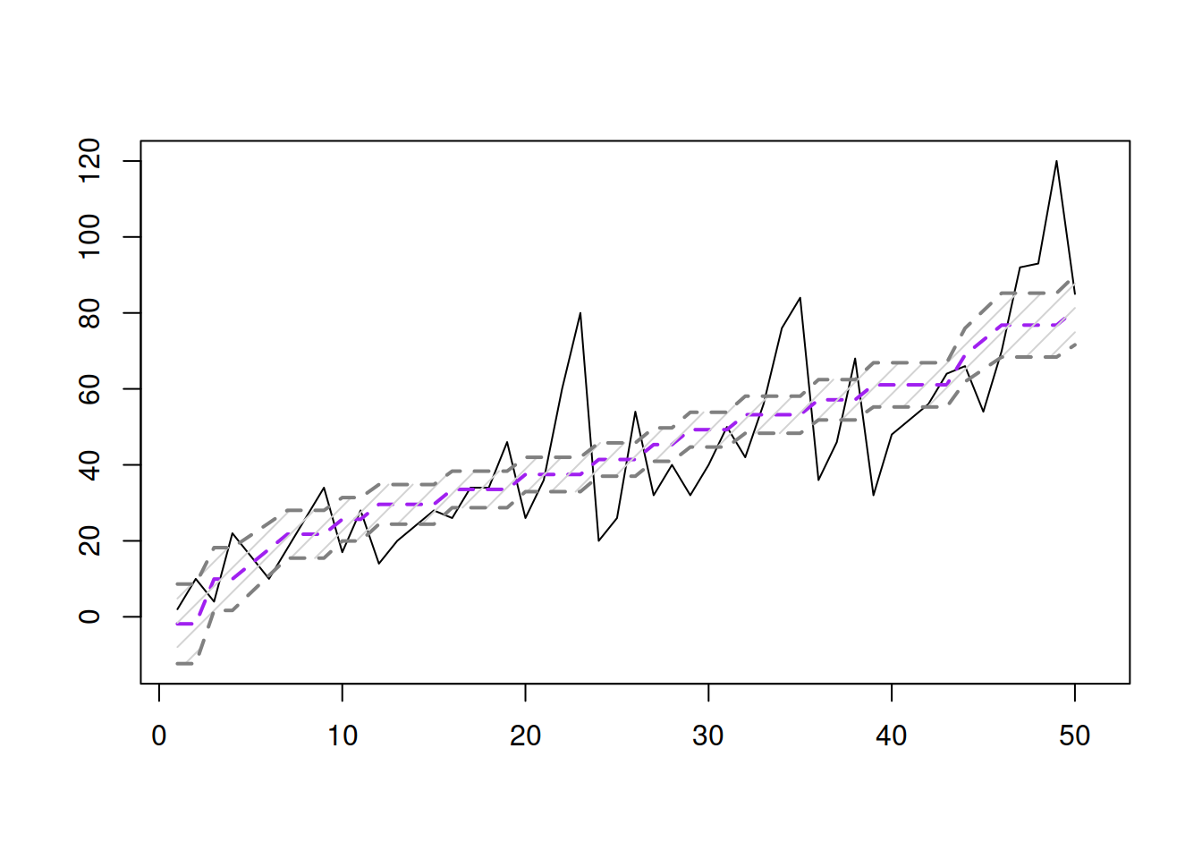
Figure 3.10: Fitted values and confidence interval for the stopping distance model.
The same fitted values and interval can be presented differently on the actuals vs fitted plot:
plot(fitted(slmSpeedDistance),actuals(slmSpeedDistance),
     xlab="Fitted",ylab="Actuals")
abline(a=0,b=1,col="blue",lwd=2)
lines(sort(fitted(slmSpeedDistance)),
      slmSpeedDistanceCI$lower[order(fitted(slmSpeedDistance))],
      col="red")
lines(sort(fitted(slmSpeedDistance)),
      slmSpeedDistanceCI$upper[order(fitted(slmSpeedDistance))],
      col="red")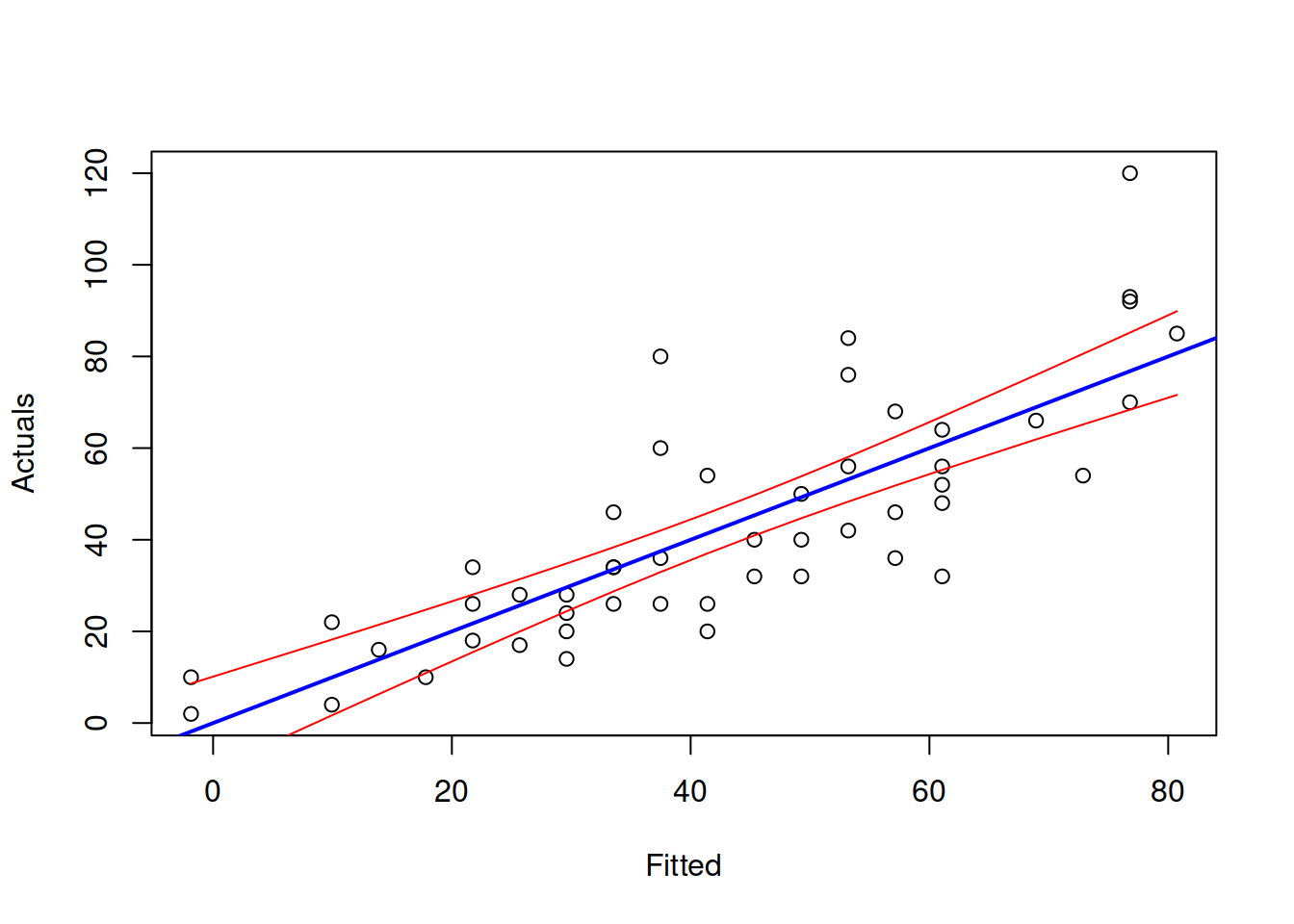
Figure 3.11: Actuals vs Fitted and confidence interval for the stopping distance model.
Figure 3.11 demonstrates the actuals vs fitted plot, together with the 95% confidence interval around the line, demonstrating where the line would be expected to be in 95% of the cases if we re-estimate the model many times. We also see that the uncertainty of the regression line is lower in the middle of the data, but expands in the tails. Conceptually, this happens because the regression line, estimated via OLS, always passes through the average point of the data \((\bar{x},\bar{y})\) and the variability in this point is lower than the variability in the tails.
If we are not interested in the uncertainty of the regression line, but rather in the uncertainty of the observations, we can refer to prediction interval. The variance in this case is: \[\begin{equation} \mathrm{V}(y_t| \mathbf{x}_t) = \mathrm{V}(\hat{a}_0 + \hat{a}_1 x_{1,t} + \hat{a}_2 x_{2,t} + \dots + \hat{a}_{k-1} x_{k-1,t} + e_t) , \tag{3.30} \end{equation}\] which can be simplified to (if assumptions of regression model hold, see Section 3.6): \[\begin{equation} \mathrm{V}(y_t| \mathbf{x}_t) = \mathrm{V}(\hat{y}_t| \mathbf{x}_t) + \hat{\sigma}^2, \tag{3.31} \end{equation}\] where \(\hat{\sigma}^2\) is the variance of the residuals \(e_t\). As we see from the formula (3.31), the variance in this case is larger than (3.28), which will result in wider interval than the confidence one. We can use normal distribution for the construction of the interval in this case (using formula similar to (3.29)), as long as we can assume that \(\epsilon_t \sim \mathcal{N}(0,\sigma^2)\).
In R, this can be done via the very same predict() function with interval="prediction":
slmSpeedDistancePI <- predict(slmSpeedDistance,interval="prediction")Based on this, we can construct graphs similar to 3.10 and 3.11.
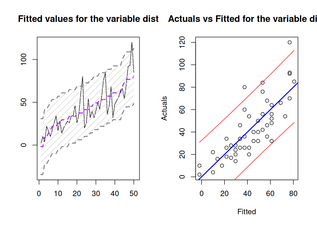
Figure 3.12: Fitted values and prediction interval for the stopping distance model.
Figure 3.12 shows the prediction interval for values over observations and for actuals vs fitted. As we see, the interval is wider in this case, covering only 95% of observations (there are 2 observations outside it).
In forecasting, prediction interval has a bigger importance than the confidence interval. This is because we are typically interested in capturing the uncertainty about the observations, not about the estimate of a line. Typically, the prediction interval would be constructed for some holdout data, which we did not have at the model estimation phase. In the example with stopping distance, we could see what would happen if the speed of a car was, for example, 30mph:
slmSpeedDistanceForecast <- predict(slmSpeedDistance,newdata=data.frame(speed=30),
                                    interval="prediction")
plot(slmSpeedDistanceForecast)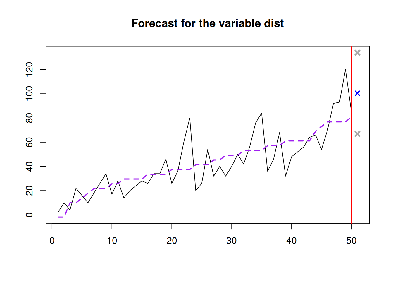
Figure 3.13: Forecast of the stopping distance for the speed of 30mph.
Figure 3.13 shows the point forecast (the expected stopping distance if the speed of car was 30mph) and the 95% prediction interval (we expect that in 95% of the cases, the cars will have the stopping distance between 66.865 and 133.921 feet.