17.2 Prediction intervals
As discussed in Section 5.2 of Svetunkov (2021c), prediction interval is needed in order to reflect the uncertainty about the data. In theory, the 95% prediction interval will cover the actual values in 95% of the cases, if it is recreated for different samples of data many time, given that the model is correctly specified. The specific formula for prediction interval will vary with the assumed distribution. For example, for the Normal distribution (assuming that \(y_{t+j} \sim \mathcal{N}(\mu_{y, t+j}, \sigma^2)\)) we will have the classical one: \[\begin{equation} y_{t+j} \in (\hat{y}_{t+j} + z_{\alpha/2} \hat{\sigma}_j^2, \hat{y}_{t+j} + z_{1-\alpha/2} \hat{\sigma}_j^2), \tag{17.1} \end{equation}\] where \(\hat{y}_{t+j}\) is the j steps ahead forecast from the model, \(\hat{\sigma}_j^2\) is the estimate of the \(j\) steps ahead variance of the error term (for example, calculated via the formula (5.11)) and \(z\) is z-statistics (providing quantile of standard normal distribution) for the selected significance level \(\alpha\). This type of prediction interval can be called parametric. It assumes a specific distribution and relies on the other assumptions about the constructed model (such as residuals are i.i.d., see Section 14). Note that the interval produced via (17.1) corresponds to two quantiles from normal distribution and can be written in a more general form as: \[\begin{equation} y_{t+j} \in \left(q \left(\hat{y}_{t+j},\hat{\sigma}_j^2,\frac{\alpha}{2}\right), q\left(\hat{y}_{t+j},\hat{\sigma}_j^2,1-\frac{\alpha}{2}\right)\right), \tag{17.2} \end{equation}\] where \(q(\cdot)\) is a quantile function of an assumed distribution, \(\hat{y}_{t+j}\) acts as a location and \(\hat{\sigma}^2\) acts as a scale of distribution. Using this general formula (17.2) for prediction intervals, we can construct them for other distributions as long as they support convolution (addition of random variables following that distribution). In ADAM framework, this works for all pure additive models that have error term that follows one of the below:
- Normal: \(\epsilon_t \sim \mathcal{N}(0, \sigma^2)\), thus \(y_{t+j} \sim \mathcal{N}(\mu_{y, t+j}, \sigma^2)\);
- Laplace: \(\epsilon_t \sim \mathcal{Laplace}(0, s)\) and \(y_{t+j} \sim \mathcal{Laplace}(\mu_{y, t+j}, s)\);
- S: \(\epsilon_t \sim \mathcal{S}(0, s)\), \(y_{t+j} \sim \mathcal{S}(\mu_{y, t+j}, s)\);
- Generalised Normal: \(\epsilon_t \sim \mathcal{GN}(0, s, \beta)\), so that \(y_{t+j} \sim \mathcal{GN}(\mu_{y, t+j}, s, \beta)\).
If a model has multiplicative components or relies on a different distribution, then the several steps ahead actual value will not necessarily follow the assumed distribution and the formula (17.2) will produce incorrect intervals. For example, if we work with a pure multiplicative ETS model, ETS(M,N,N), assuming that \(\epsilon_t \sim \mathcal{N}(0, \sigma^2)\), the 2 steps ahead actual value will be expressed via the past values as: \[\begin{equation} y_{t+2} = l_{t+1} (1+\epsilon_{t+2}) = l_{t} (1+\alpha \epsilon_{t+1}) (1+\epsilon_{t+2}) , \tag{17.3} \end{equation}\] which introduces the product of normal distributions and thus \(y_{t+2}\) does not follow Normal distribution any more. In those cases, we might have several options of what to use in order to produce intervals. They are discussed in the subsections below.
17.2.1 Approximate
Even if the actual multisteps value does not follow the assumed distribution, in some cases we can use approximations: the produced prediction interval will not be too far from the correct one. The main idea behind the approximate intervals is to rely on the same distribution for \(y_{t+j}\) as for the error term, even though we know that the variable will not follow it. In case of multiplicative error models, the limit (6.5) can be used to motivate the usage of that assumption. For example, in case of the ETS(M,N,N) model, we know that \(y_{t+2}\) will not follow normal distribution, but if the variance of the error term is low (e.g. \(\sigma^2 < 0.05\)) and the smoothing parameter \(\alpha\) is close to zero, then the normal distribution would be a fine approximation of the real one. This will become clear, if we expand the brackets in (17.3): \[\begin{equation} y_{t+2} = l_{t} (1 + \alpha \epsilon_{t+1} + \epsilon_{t+2} + \alpha \epsilon_{t+1} \epsilon_{t+2}) . \tag{17.4} \end{equation}\] With the conditions discussed above (low \(\alpha\), low variance) the term \(\alpha \epsilon_{t+1} \epsilon_{t+2}\) will be close to zero, thus making the sum of normal distributions dominate in the formula (17.4). The advantage of this approach is in its speed: you only need to know the scale parameter of the error term and the conditional location (e.g. conditional expectation). The disadvantage of the approach is that it becomes inaccurate with the increase of parameters and scale of the model. The rule of thumb, when to use this approach: if the smoothing parameters are all below 0.1 (in case of ARIMA this is equivalent to MA terms being negative and AR terms being close to zero) or the scale of distribution is below 0.05, the differences between the proper interval and the approximate one should be negligible.
17.2.2 Simulated
This approach relies on the idea discussed in Section 17.1.1. It is universal and supports any distribution, because it only assumes that the error term follows a distribution (no need for the actual value to do that as well), and the simulate paths are produced based on the generated values and assumed model. After generating \(n\) paths, one can take the desired quantiles to get the bounds of the interval. The main issue of the approach is that it is time consuming (slower than the approximate intervals) and might be highly inaccurate if the number of iterations \(n\) is low. This approach is used as a default in adam() for the non-additive models.
17.2.3 Semiparametric
The three approaches above assume that the residuals of the applied model are i.i.d.. If this assumption is violated (for example, the residuals are autocorrelated), then the intervals might be miscalibrated (i.e. producing wrong values). In this case, we might need to use different approaches. One of this is the construction of semiparametric prediction intervals. This approach relies on the in-sample multistep forecast errors, discussed in Section 14.7.1. After producing \(e_{t+j|t}\) for all in sample values of \(t\) and for \(j=1,\dots,h\), we can use these errors to calculate the respective h steps ahead conditional variances \(\sigma_j^2\) for \(j=1,\dots,h\). These values can then be inserted in the formula (17.2) to get the desired prediction intervals. The approach works well in case of pure additive models, as it relies on specific assumed distribution. However, it might have limitations similar to those discussed earlier for the mixed models and for the models with positively defined distributions (such as Log Normal, Gamma and Inverse Gaussian).
17.2.4 Nonparametric
In the cases, when some of assumptions might be violated and when we cannot rely on the parametric distributions, we can use nonparametric approach, proposed by Taylor and Bunn (1999). The authors proposed using the multistep forecast errors in order to construct the following quantile regression model: \[\begin{equation} \hat{e}_{t+j} = a_0 + a_1 j + a_2 j^2, \tag{17.5} \end{equation}\] for each of the bounds of the interval. The motivation behind the polynomial in (17.5) is because typically the multisteps conditional variance will involve square of forecast horizon. The main issue with this approach is that the polynomial has an extremum, which might appear sometime in the future, so, for example, the upper bound of the interval would increase until that point and then start decreasing. In order to overcome this limitation, I propose using the power function instead: \[\begin{equation} \hat{e}_{t+j} = a_0 j^a_1 . \tag{17.6} \end{equation}\] This way, the bounds will always change monotonically, and the parameter \(a_1\) will control the speed of expansion of the interval. The model (17.6) is estimated using quantile regression for the upper and the lower bounds separately as Taylor and Bunn (1999) recommend. This approach does not require any assumptions about the model and works as long as there is enough observations in sample (so that the matrix of forecast errors contains more rows than columns). The main limitation of this approach is that it relies on quantile regression and thus will have the same issues as, for example, pinball score has (see discussion in Section 2.2): the quantiles are not always uniquely defined. Another limitation is that we assume that the quantiles will follow the model (17.6), which might be violated in some real life cases.
17.2.5 Empirical
Another alternative to the parametric intervals uses the same matrix of multistep forecast errors as discussed earlier. The empirical approach is simpler than the approaches discussed above and does not rely on any assumptions. The idea behind it is to just take quantiles of the forecast errors for each forecast horizon \(j=1,\dots,h\). These quantiles are then added to the point forecast if the error term is additive or are multiplied by it in case of the multiplicative one. (Kourentzes2021TBA?) show that the empirical prediction intervals perform on average better than the other approaches. So, in general I would recommend producing empirical intervals if it was not for the computational difficulties related to the multistep forecast errors: if you have an additive model and believe that the assumptions are satisfied, then parametric interval will be as accurate, but faster. Furthermore, in cases of small samples, the approach will be unreliable due to the same problem with quantiles discussed earlier.
17.2.6 Complete parametric
So far, all the intervals discussed above relied on an unrealistic assumption that the parameters of the model are known. This is one of the reasons, why the intervals produced for ARIMA and ETS are typically narrower than expected (see, for example results of competition in Athanasopoulos et al., 2011). But as we discussed in Section 16, there are ways of capturing the uncertainty of estimated parameters of the model and propagating it to the future uncertainty (i.e. to conditional h steps ahead variance). As discussed in Section 16.4, the more general approach is to create many in-sample model paths based on randomly generated parameters of the model. This way we can obtain a variety of states for the final in-sample observation \(T\) and then use those values in the construction of final prediction intervals. The simplest and most general way of producing intervals in this case is using simulations (as discussed earlier in Subsection 17.2.2). The intervals produced via this approach will be wider than the conventional ones, and their width will be proportional to the uncertainty around the parameters. This also means that the intervals might become too wide if the uncertainty is not captured correctly (see discussion in Section 16.4). One of the main limitations of the approach is its computational time: it will be proportional to the number of simulation paths for both refitted model and prediction intervals.
It is also theoretically possible to use other approaches for the intervals construction (e.g. “empirical” one for each of the set of parameters of the model), but they would be even more computationally expensive than the approach described above and will have the limitations as discussed above (i.e. non-uniqueness of quantiles, sample size requirements).
17.2.7 Explanatory variables
In all the cases described above, when constructing prediction intervals for model with explanatory variables, we would assume that their values are known in the future. Even if they are note provided by the user and need to be forecasted, the produced conditional expectations will be used for all the calculations. This is not entirely correct approach as was shown in Section 10.2.2, but it speeds up the calculation process and typically produces adequate results.
17.2.8 Example in R
All the types of intervals discussed in this Section are implemented for the adam() models in smooth package. In order to demonstrate how they work and differ we consider the example with ETS model on BJSales data:
adamModel <- adam(BJsales, h=10, holdout=TRUE)
modelType(adamModel)
## [1] "AAdN"The model selected above is ETS(A,Ad,N). In order to make sure that the parametric intervals are suitable, we can do model diagnostics (see Section 14), shown in Figure 17.2.
par(mfcol=c(2,3))
plot(adamModel,c(2,4,6,8,10:11))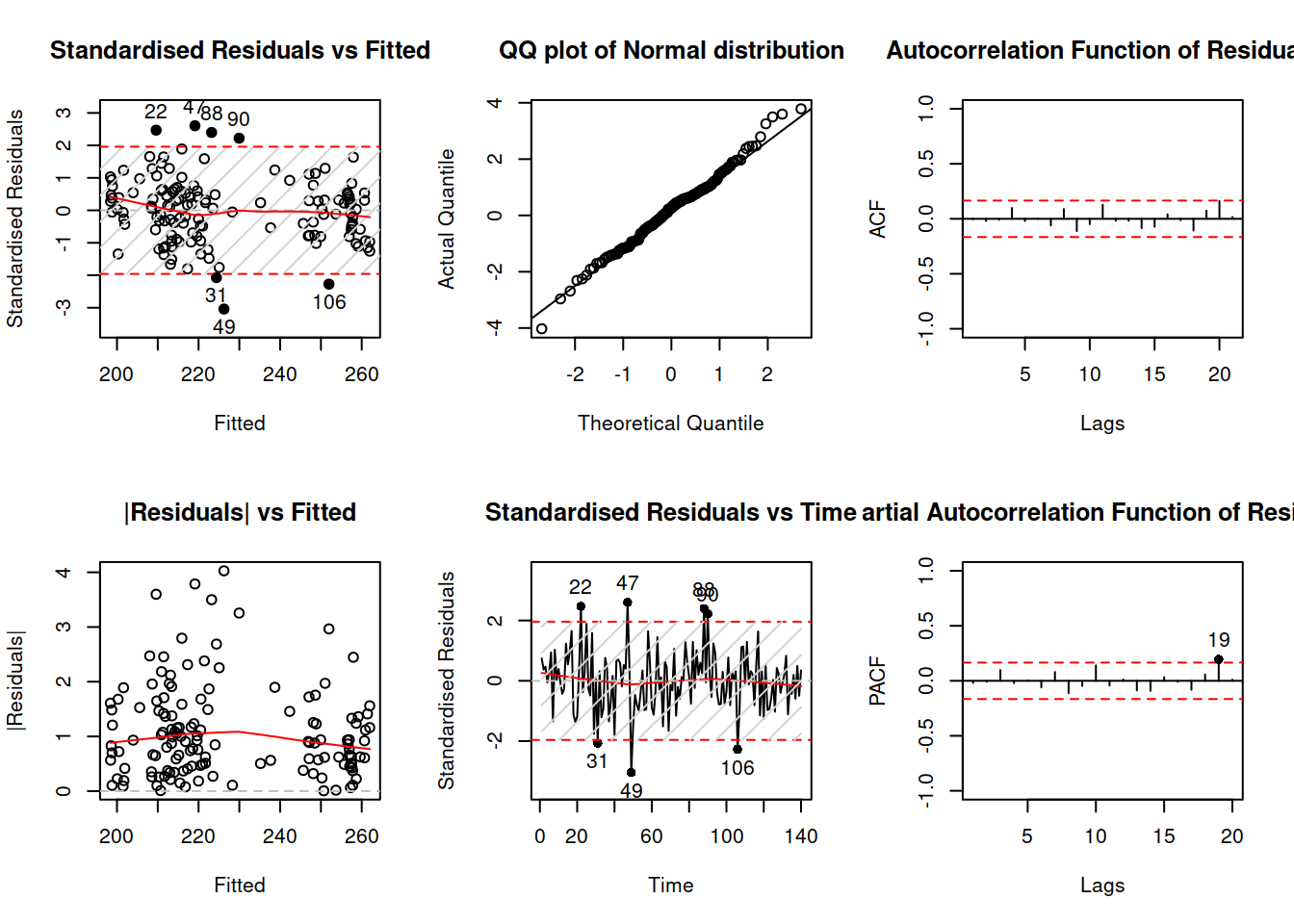
Figure 17.2: Diagnostics of the ADAM model on BJSales data.
The residuals of the model do not exhibit any serious issues, so, given that this is pure additive model, we can conclude that the parametric intervals would be appropriate for this situation and produce the plot with them (see Figure 17.3).
plot(forecast(adamModel,h=10,interval="parametric"))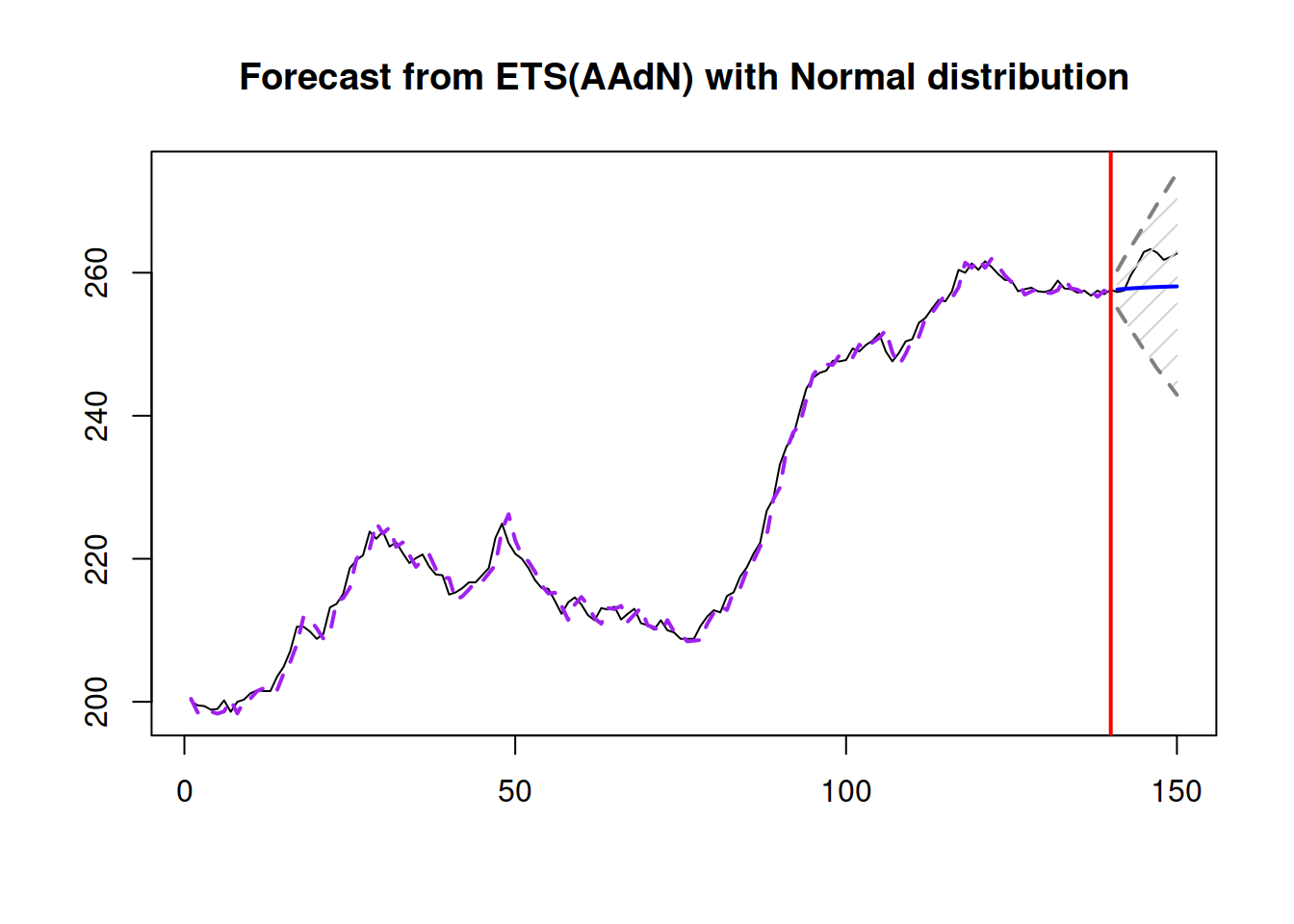
Figure 17.3: Parametric prediction intervals for ADAM on BJSales data.
The only thing that these intervals do not take into account is the uncertainty about the parameters, so we can construct the respective intervals either via reforecast() function or using the same forecast(), but with the option interval="complete". Note that this is a computationally expensive operation (both in terms of time and memory), so the more iterations you set up, the longer it will take and more memory it will consume.
plot(forecast(adamModel,h=10,interval="complete",nsim=100))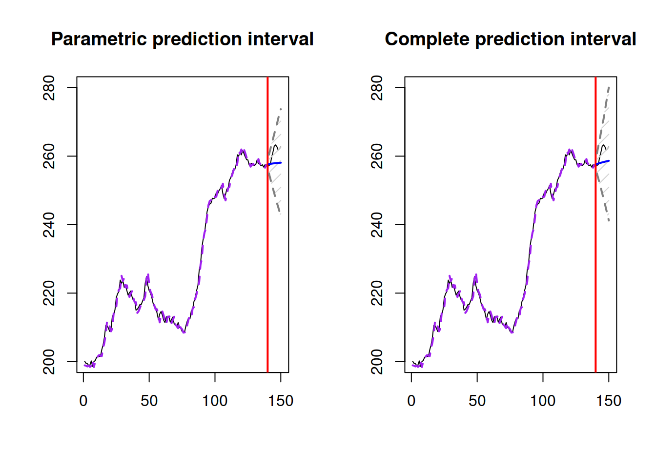
Figure 17.4: Parametric prediction intervals for ADAM on BJSales data.
The resulting complete parametric interval shown in Figure 17.4, will not be substantially different from the parametric one. This is because the smoothing parameters of the model are high, thus the model forgets the initial states fast and the uncertainty does not propagate to the last observation as much as in the case of lower values of parameters:
summary(adamModel)##
## Model estimated using adam() function: ETS(AAdN)
## Response variable: BJsales
## Distribution used in the estimation: Normal
## Loss function type: likelihood; Loss function value: 240.3777
## Coefficients:
## Estimate Std. Error Lower 2.5% Upper 97.5%
## alpha 0.9764 0.1053 0.7682 1.0000 *
## beta 0.2544 0.0929 0.0706 0.4380 *
## phi 0.8922 0.0645 0.7646 1.0000 *
## level 201.3166 2.5834 196.2071 206.4223 *
## trend -0.8043 1.5771 -3.9235 2.3125
##
## Sample size: 140
## Number of estimated parameters: 6
## Number of degrees of freedom: 134
## Information criteria:
## AIC AICc BIC BICc
## 492.7554 493.3870 510.4053 511.9658Figure 17.5 demonstrates what happens with the fitted values, when we take the uncertainty into account.
plot(refit(adamModel))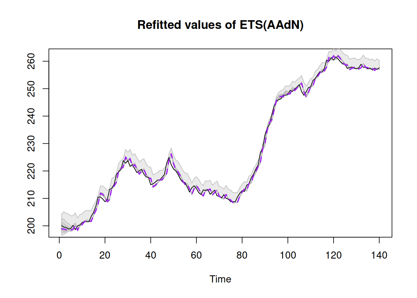
Figure 17.5: Refitted values for ADAM on BJSales data.
In order to make things more complicated and interesting, we introduce explanatory variable with lags and leads of the indicator BJsales.lead:
BJsalesData <- cbind(as.data.frame(BJsales),xregExpander(BJsales.lead,c(-3:3)))
colnames(BJsalesData)[1] <- "y"
adamModelX <- adam(BJsalesData, "YYY", h=10, holdout=TRUE, regressors="select")
In order to make the task more complicated, I have asked the function specifically to do the selection between pure multiplicative models (see Section 15.1). In this case, we will construct several different types of prediction intervals and compare them:
adamModelPI <- vector("list",6)
intervalType <- c("approximate","semiparametric","nonparametric","simulated","empirical","complete")
for(i in 1:6){
  adamModelPI[[i]] <- forecast(adamModelX,h=10,interval=intervalType[i])
}
## Warning: The covariance matrix of parameters is not positive semi-definite. I
## will try fixing this, but it might make sense re-estimating adam(), tuning the
## optimiser.These can be plotted in one Figure 17.6.
par(mfcol=c(3,2))
for(i in 1:6){
  plot(adamModelPI[[i]],main=paste0(intervalType[i]," interval"))
}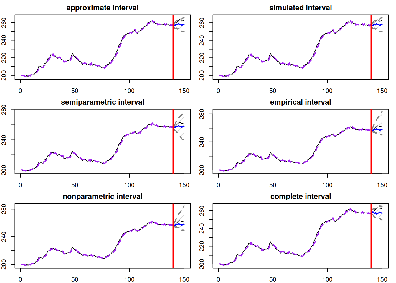
Figure 17.6: Different prediction intervals for ADAM ETS(M,N,N) on BJSales data
The thing to notice is how the width and shape of intervals change depending on the used approach. The approximate and simulated intervals look very similar, because the selected model is ETSX(M,N,N) with standard error of 0.005 (thus the approximation works well). The complete interval is similar as well because the estimated smoothing parameters \(\alpha=1\) (thus the forgetting happens instantaneously). It has a slightly different shape because the number of iterations for the interval was low (nsim=100 for interval="complete" by default). The semiparametric interval is the widest as it calculates the forecast errors directly, but still uses the normal approximation. Both nonparametric and empirical are skewed, because the in-sample forecast errors followed skewed distributions (see Figure 17.7).
adamModelXForecastErrors <- rmultistep(adamModelX,h=10)
boxplot(adamModelXForecastErrors)
abline(h=0,col="red")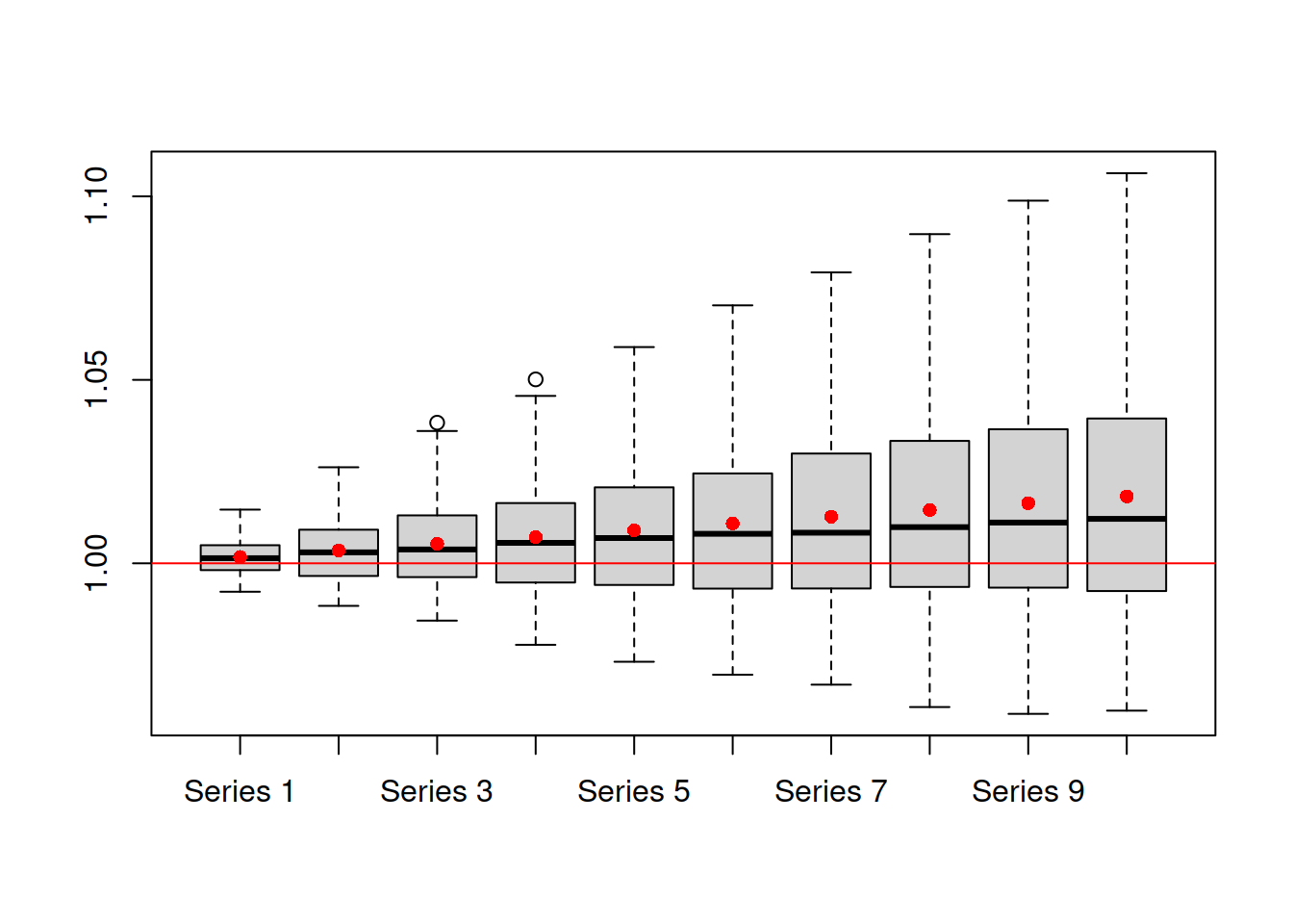
Figure 17.7: Distribution of in-sample multistep forecast errors from ADAM ETSX(M,N,N) model on BJSales data.
Analysing the plot 17.6, it might be difficult to select the most appropriate type of prediction interval. But the model diagnostics (Section 14) might help in this situation:
- If the residuals look i.i.d. and model does not omit important variables, then choose between parametric approximate and simulated intervals, choose:
- “parametric” in case of pure additive model,
- “approximate” in other cases, when the standard error is lower than 0.05 or smoothing parameters are close to zero,
- “simulated” if you deal with non-additive model with high values of standard error and smoothing parameters,
- “complete parametric” when the smoothing parameters of the model are close to zero, and you want to take the uncertainty about the parameters into account;
- If residuals seem to follow the assumed distribution, but are not i.i.d., then “semiparametric” approach might help. Note that this only works on samples of \(T>>h\);
- If residuals do not follow the assumed distribution, but your sample is still longer than the forecast horizon, then use either “empirical” or “nonparametric” intervals.
Finally, forecast.adam() will automatically select between “parametric,” “approximate” and “simulated” if you ask for interval="prediction".