


UPDATE: Starting from smooth v 3.0.0, the occurrence part of the model has been removed from es() and other functions. The only one that implements this now is adam(). This post has been updated on 01 January 2021.
UPDATE: Starting from smooth v 2.5.0, the model and the respective functions have changed. Now instead of calling the parameter intermittent and working with iss(), one needs to use occurrence and oes() respectively. This post has been updated on 25 April 2019.
One of the features of functions of smooth package is the ability to work with intermittent data and the data with periodically occurring zeroes.
Intermittent time series is a series that has non-zero values occurring at irregular frequency (Svetuknov and Boylan, 2017). Imagine retailer who sells green lipsticks. The demand on such a product will not be easy to predict, because green colour is not a popular colour in this case, and thus the data of sales will contain a lot of zeroes with seldom non-zero values. Such demand is called “intermittent”. In fact, many products exhibit intermittent patterns in sales, especially when we increase the frequency of measurement (how many tomatoes and how often does a store sell per day? What about per hour? Per minute?).
The other case is when watermelons are sold in high quantities over summer and are either not sold at all or sold very seldom in winter. In this case the demand might be intermittent or even absent in winter and have a nature of continuous demand during summer.
smooth functions can work with both of these types of data, building upon mixture distributions.
In this post we will discuss the basic intermittent demand statistical models implemented in the package.
The model
First, it is worth pointing out that the approach that is used in the statistical methods and models discussed in this post assumes that the final demand on the product can be split into two parts (Croston, 1972):
- Demand occurrence part, which is represented by a binary variable, which is equal to one when there is a non-zero demand in period \(t\) and zero otherwise;
- Demand sizes part, which reflects the amount of sold product when demand occurrence part is equal to one.
This can be represented mathematically by the following equation:
\begin{equation} \label{eq:iSS}
y_t = o_t z_t ,
\end{equation}
where \(o_t\) is the binary demand occurrence variable, \(z_t\) is the demand sizes variable and \(y_t\) is the final demand. This equation was originally proposed by Croston, (1972), although he has never considered the complete statistical model and only proposed a forecasting method.
There are several intermittent demand methods that are usually discussed in forecasting literature: Croston (Croston, 1972), SBA (Syntetos & Boylan, 2000) and TSB (Teunter et al., 2011). These are good methods that work well in intermittent demand context (see, for example, Kourentzes, 2014). The only limitation is that they are the “methods” and not “models”. Having models becomes important when you want to include additional components and produce proper prediction intervals, need the ability to select the appropriate components and do proper statistical inference. So, John Boylan and I developed the model underlying these methods (Svetunkov & Boylan, 2017), based on \eqref{eq:iSS}. It is built upon ETS framework, so we call it “iETS”. Given that all the intermittent demand forecasting methods rely on simple exponential smoothing (SES), we suggested to use ETS(M,N,N) model for both demand sizes and demand occurrence parts, because it underlies SES (Hyndman et al., 2008). One of the key assumptions in our model is that demand sizes and demand occurrences are independent of each other. Although, this is an obvious simplification, it is inherited from Croston and TSB, and seems to work well in many contexts.
The iETS(M,N,N) model, discussed in our paper is formulated the following way:
\begin{equation}
\begin{matrix} \label{eq:iETS}
y_t = o_t z_t \\
z_t = l_{z,t-1} \left(1 + \epsilon_t \right) \\
l_{z,t} = l_{z,t-1}( 1 + \alpha_z \epsilon_t) \\
o_t \sim \text{Bernoulli}(p_t)
\end{matrix} ,
\end{equation}
where \(z_t\) is represented by the ETS(M,N,N) model, \(l_{z,t}\) is the level of demand sizes, \(\alpha_z\) is the smoothing parameter and \(\epsilon_t\) is the error term. The important assumption in our implementation of the model is that \(\left(1 + \epsilon_t \right) \sim \text{log}\mathcal{N}(0, \sigma_\epsilon^2) \) – something that we discussed in one of the previous posts. This means that the demand will always be positive. However if you deal with some other type of data, where negative values are natural, then you might want to stick with pure additive model.
Having this statistical model, makes it extendable, so that one can add trend, seasonal component, or exogenous variables. We don’t discuss these elements in our paper, but it is briefly mentioned in the conclusions. And we don’t discuss these features just yet, we will cover them in the next post.
Now the main question that stays unanswered is how to model the probability \(p_t\). And there are several approaches to that:
- iETS\(_F\) – assume that the demand occurs at random with a fixed probability (so \(p_t = p\)).
- iETS\(_O\) – so called “Odds Ratio” model, which uses the logistic curve in order to update the probability. In this case the model is focused on the probability of occurrence of the demand.
- iETS\(_I\) – the “Inverse Odds Ratio” model, which uses similar principles to iETS\(_O\), but focusing on the probability of non-occurrence. This model underlies Croston (1972) method, but it uses different principles. Instead of updating the probability only when demand occurs, it does that on every observation.
- iETS\(_D\) – the “Direct probability” model, which uses the principles, suggested by Teunter et al., (2011). In this case the probability is updated directly based on the values of occurrence variable, using SES method.
- iETS\(_G\) – the “General” model, encompassing all above. This model has two sub-models for the demand occurrence, capturing both the probability of occurrence and non-occurrence.
In case (1) the model is very basic, and we can just estimate the value of probability and produce forecasts. In cases of (2) – (5), we suggest using another ETS(M,N,N) model as underlying each of these processes. So when it comes to producing forecasts, in both cases we assume that future level of probability will be the same as the last obtained one (level forecast from the local-level model). After that the final forecast is generated using:
\begin{equation} \label{eq:iSSForecast}
\hat{y}_t = \hat{p}_t \hat{z}_t ,
\end{equation}
where \(\hat{p}_t\) is the forecast of the probability, \(\hat{z}_t\) is the forecast of demand sizes and \(\hat{y}_t\) is the final forecast of the intermittent demand.
In order to distinguish the whole model \eqref{eq:iETS}, the demand sizes and the demand occurrence parts of the model, different names are used. For example, iETS\(_G\)(M,N,N) would refer to the full model \eqref{eq:iETS}, (\(y_t\)), oETS\(_G\)(M,N,N) would refer to the occurrence part of the model (\(o_t\)) and ETS(M,N,N) refers to the demand sizes part (\(z_t\)). In all these three cases the “(M,N,N)” part indicates that the exponential smoothing with multiplicative error, no trend and no seasonality is used. The more advanced notations for the iETS models are available, but they will be discuss in the next post. For now we will stick with the level models and use the shorter names.
Summarising advantages of our framework:
- Our model is extendable: you can use any ETS model and even introduce exogenous variables. This is already available in smooth package. In fact, you can use any model you want for demand sizes and a wide variety of models for demand occurrence variable;
- The model allows selecting between the aforementioned types of intermittent models (“fixed” / “odds ratio” / “inverse odds ratio” / “direct” and “general”) using information criteria. This mechanism works fine on large samples, but, unfortunately, does not always work well in cases of small samples;
- The model allows producing prediction intervals for several steps ahead and cumulative (over a lead time) upper bound of the intervals. The latter arises naturally from the model and can be used for safety stock calculation;
- The estimation of models is done using likelihood function and not some ad-hoc estimators. This means that the estimates of parameters become efficient and consistent;
- Although the proposed model is continuous, we show in our paper that it is more accurate than several other integer-valued models. Still, if you want to have integer numbers as your final forecasts, you can round up or round down either the point or prediction intervals, ending up with meaningful values. This can be done due to a connection between the quantiles of rounded values and the rounding of quantiles of continuous variable (discussed in Appendix of our paper).
If you need more details, have a look at our working paper (have I already advertise it enough in this post?).
Implementation. Demand occurrence
The aforementioned model with different occurrence types is available in smooth package. There is a special function for demand occurrence part, called oes() (Occurrence Exponential Smoothing) and there is a parameter in every smooth forecasting function called occurrence, which can be one of: “none”, “fixed”, “odds-ratio”, “inverse-odds-ratio”, “direct”, “general” or “auto”, corresponding to the sub types of oETS discussed above. The “auto” option selects the best occurrence model of the five. For now we will neglect this option and come back to it later.
So, let’s consider an example with artificial data. We create the following time series:
x <- c(rpois(25,5),rpois(25,1),rpois(25,0.5),rpois(25,0.1))
This way we have an artificial data, where both demand sizes and demand occurrence probability decrease over time in a step-wise manner, each 25 observations. The generated data resembles something called "demand obsolescence" or "dying out demand". Let’s start by fitting those five models for the demand occurrence part:
oesFixed <- oes(x, occurrence="f", h=25)
Occurrence state space model estimated: Fixed probability
Underlying ETS model: oETS[F](MNN)
Smoothing parameters:
level
    0
Vector of initials:
level
 0.55
Information criteria:
     AIC     AICc      BIC     BICc
139.6278 139.6686 142.2329 142.3269
oesOdds <- oes(x, occurrence="o", h=25)
Occurrence state space model estimated: Odds ratio
Underlying ETS model: oETS[O](MNN)
Smoothing parameters:
level
0.828
Vector of initials:
 level
14.442
Information criteria:
     AIC     AICc      BIC     BICc
116.3124 116.4361 121.5227 121.8076
oesInverse <- oes(x, occurrence="i", h=25)
Occurrence state space model estimated: Inverse odds ratio
Underlying ETS model: oETS[I](MNN)
Smoothing parameters:
level
0.116
Vector of initials:
level
0.039
Information criteria:
     AIC     AICc      BIC     BICc
 98.5508  98.6745 103.7611 104.0460
oesDirect <- oes(x, occurrence="d", h=25)
Occurrence state space model estimated: Direct probability
Underlying ETS model: oETS[D](MNN)
Smoothing parameters:
level
0.115
Vector of initials:
level
0.884
Information criteria:
     AIC     AICc      BIC     BICc
106.5982 106.7219 111.8086 112.0934
oesGeneral <- oes(x, occurrence="g", h=25)
Occurrence state space model estimated: General
Underlying ETS model: oETS[G](MNN)(MNN)
Information criteria:
     AIC     AICc      BIC     BICc
102.5508 102.9718 112.9715 113.9410
By looking at the outputs, we can already say that oETS\(_I\) model performs better than the others in terms of information criteria - it has the lowest AIC, as well as the other criteria. This is because this model is more suitable for cases, when demand is dying out, as it focuses on demand non-occurrence. Note that the optimal smoothing parameter for the oETS\(_O\) is quite high. This is because the model is more focused on demand occurrences. If the demand was building out, not dying out in our example, the situation would be different: the oETS\(_O\) would have a lower parameter and oETS\(_I\) would have the higher one. Note that the initial level of oETS\(_I\) is equal to 0.116, which corresponds to \(\frac{1}{1+0.116} \approx 0.89\), which is the probability of occurrence at the beginning of time series.
Note also, that the oETS\(_G\) does not print out details, because it has two models (called modelA and modelB in R), each of which has their own parameters. Here are the outputs of both these models:
oesGeneral$modelA
oesGeneral$modelB
Occurrence state space model estimated: General
Underlying ETS model: oETS(MNN)_A
Smoothing parameters:
level
    0
Vector of initials:
level
   16
Information criteria:
     AIC     AICc      BIC     BICc
 98.5508  98.6745 103.7611 104.0460

Occurrence state space model estimated: General
Underlying ETS model: oETS(MNN)_B
Smoothing parameters:
level
0.116
Vector of initials:
level
0.628
Information criteria:
     AIC     AICc      BIC     BICc
 98.5508  98.6745 103.7611 104.0460
Note that oETS\(_G\) and both models A and B have the same likelihood, because they are all parts of one and the same thing. However, the information criteria differ because they have different number of parameters to estimate: models A and B have 2 parameters each, which means that the whole model has 4 parameters. Also, note that the model A has the smoothing parameter equal to zero, which means that there is no updated of states in that part of model. We will come back to this observation in a moment.
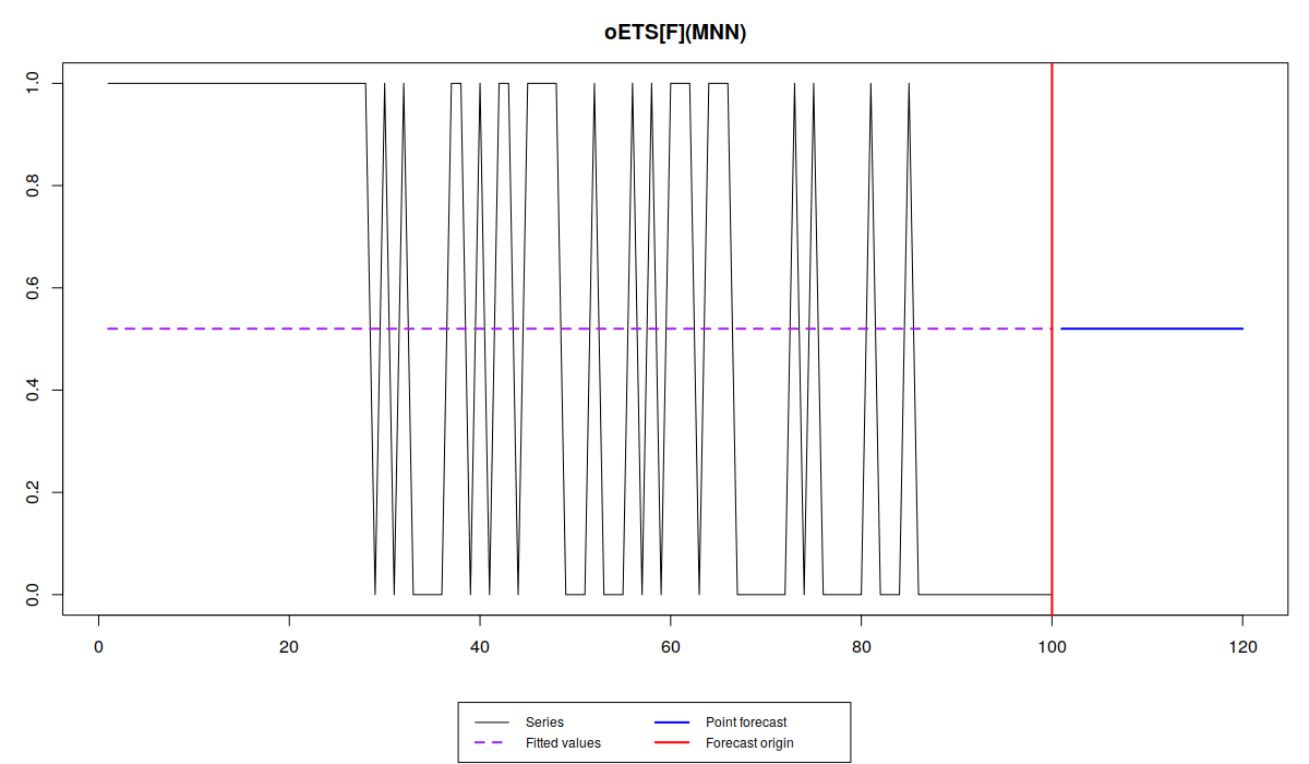
We can also plot the actual occurrence variable, fitted and forecasted probabilities using plot function:
plot(oesFixed)
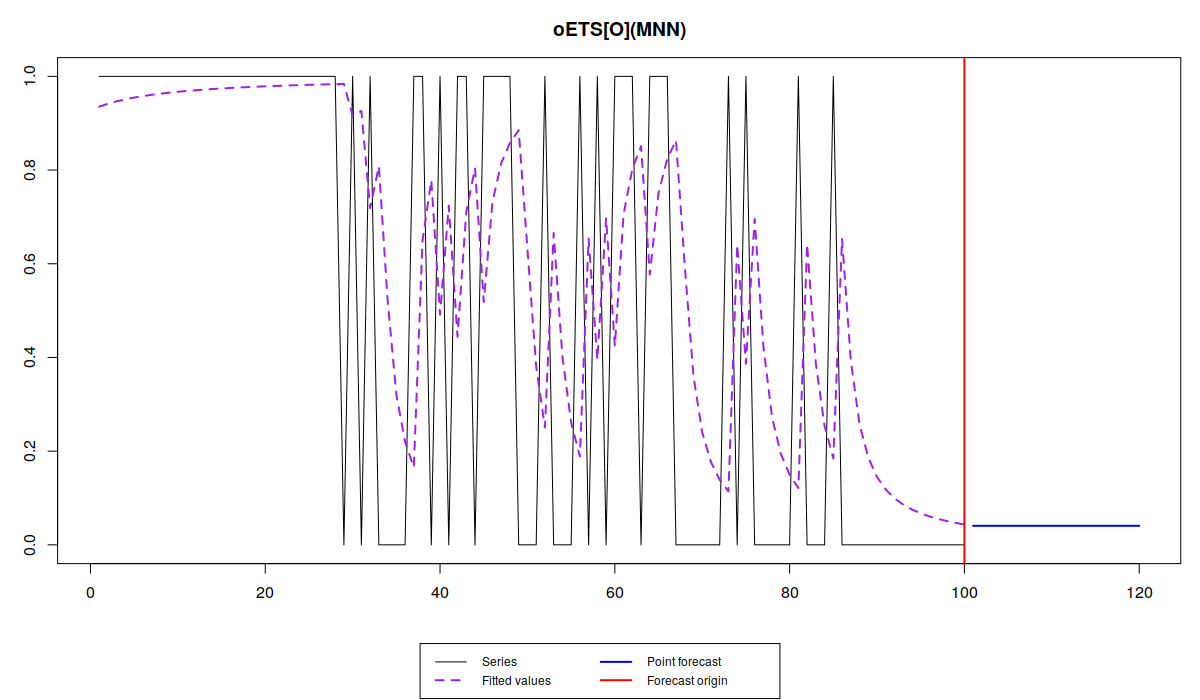
plot(oesOdds)
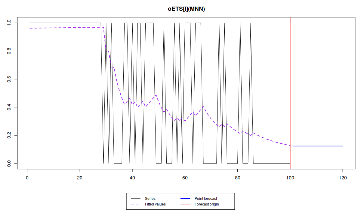
plot(oesInverse)
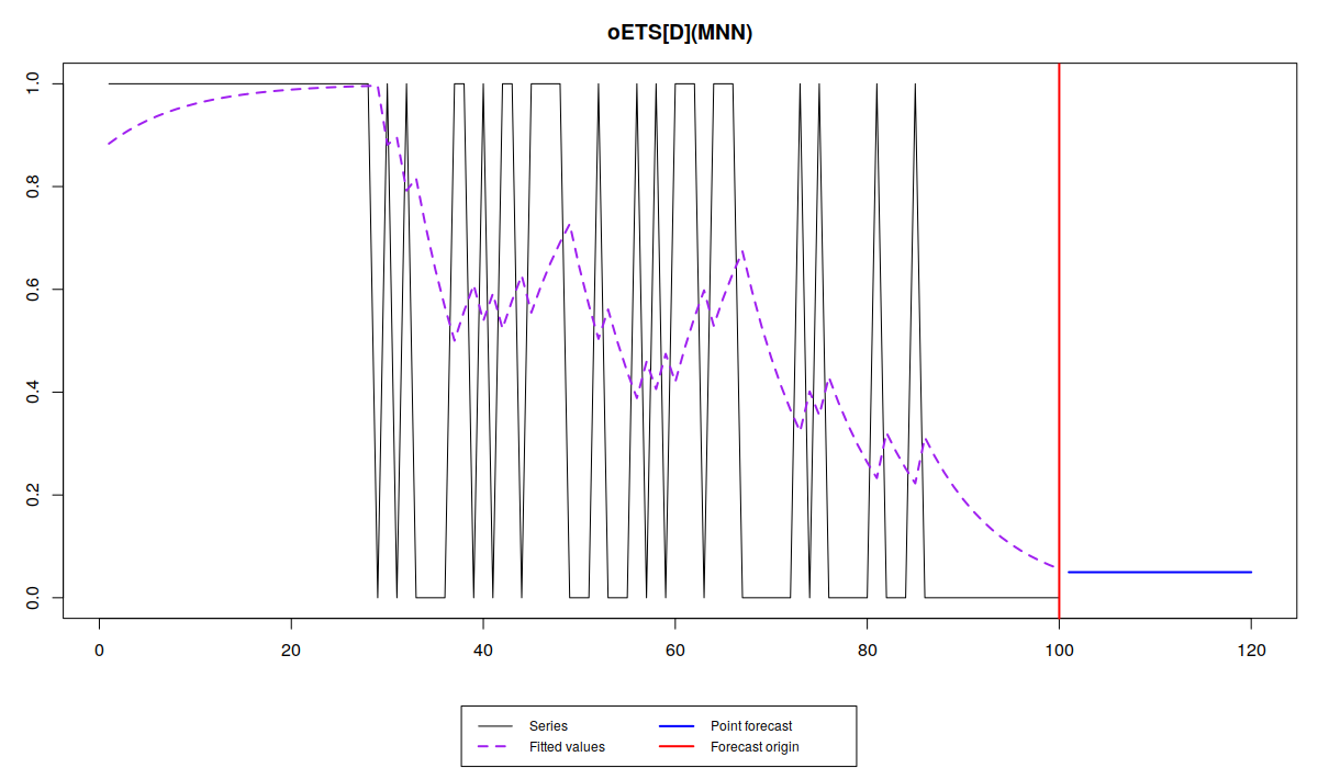
plot(oesDirect)
plot(oesGeneral)
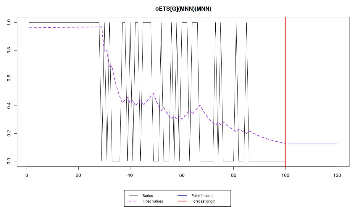
Note that the different models capture the probability differently. While oETS\(_F\) averages out the probability, all the other models react to the changes in the data, but differently:
odds ratio model is more reactive and seems not to do a good job, trying to keep up after the changes in the data; inverse odds ratio is much smoother; the direct probability model is more reactive, but not as reactive as the odds ratio one; finally the general model replicates the behaviour of the inverse odds ratio model. The latter happens because, as we have seen from the output above, model A in oETS\(_G\) is not updating the states, which means that the general and more complicated model reverts to the special case of oETS\(_I\). Still, it is worth mentioning that all the models predict that the probability will be quite low, which corresponds to the data that we have generated.
Although we could have tried out the more complicated ETS models for the demand occurrence, we will leave this to the next post.
Implementation. The whole demand
In order to deal with the intermittent data and produce the forecasts for the whole time series, we can use either es(), or ssarima(), or ces(), or gum() - all of them have the parameter occurrence, which is equal to "none" by default. We will use an example of ETS models. In order to simplify things we will use iETS\(_I\) model (because we have noticed that it is more appropriate for the data than the other models):
es(x, "MNN", occurrence="i", silent=FALSE, h=25)
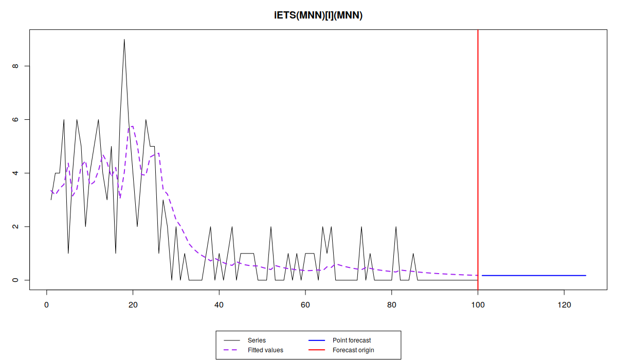
The forecast of this model is a straight line, close to zero due to the decrease in both demand sizes and demand occurrence parts. However, knowing that the demand decreases, we can use trend model in this case. And the flexibility of the approach allows us doing that, so we fit ETS(M,M,N) to demand sizes:
es(x, "MMN", occurrence="i", silent=FALSE, h=25)
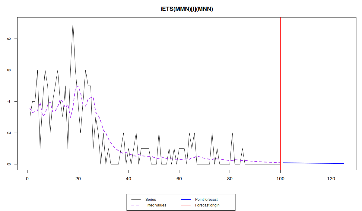
The forecast in this case is even closer to zero and reaches it asymptotically, which means that we foresee that the demand on our product will on average die out.
We can also produce prediction intervals and use model selection for demand sizes. If you know that the data cannot be negative (e.g. selling tomatoes in kilograms), then I would recommend using the pure multiplicative model:
es(x, "YYN", occurrence="i", silent=FALSE, h=25, intervals=TRUE)
Forming the pool of models based on... MNN, MMN, Estimation progress: 100%... Done!
Time elapsed: 1.02 seconds
Model estimated: iETS(MMN)
Occurrence model type: Inverse odds ratio
Persistence vector g:
alpha  beta
0.268 0.000
Initial values were optimised.
7 parameters were estimated in the process
Residuals standard deviation: 0.386
Cost function type: MSE; Cost function value: 0.149

Information criteria:
     AIC     AICc      BIC     BICc
333.4377 334.0760 348.5648 339.9301
95% parametric prediction intervals were constructed
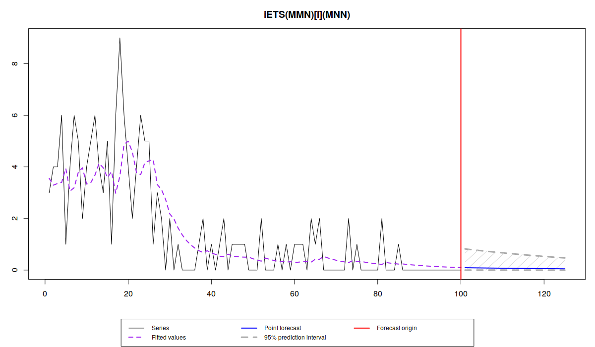
As we can see, the multiplicative trend model appears to be more suitable for our data. Note that the prediction intervals for the model are narrowing down, which is due to the decrease of level of demand. Compare this graph with the one when the pure additive model is selected:
es(x, "XXN", occurrence="i", silent=FALSE, h=25, intervals=TRUE)
Forming the pool of models based on... ANN, AAN, Estimation progress:    ... Done!
Time elapsed: 0.23 seconds
Model estimated: iETS(ANN)
Occurrence model type: Inverse odds ratio
Persistence vector g:
alpha
0.251
Initial values were optimised.
5 parameters were estimated in the process
Residuals standard deviation: 1.125
Cost function type: MSE; Cost function value: 1.265

Information criteria:
     AIC     AICc      BIC     BICc
459.8706 460.1206 472.8964 464.2617
95% parametric prediction intervals were constructed
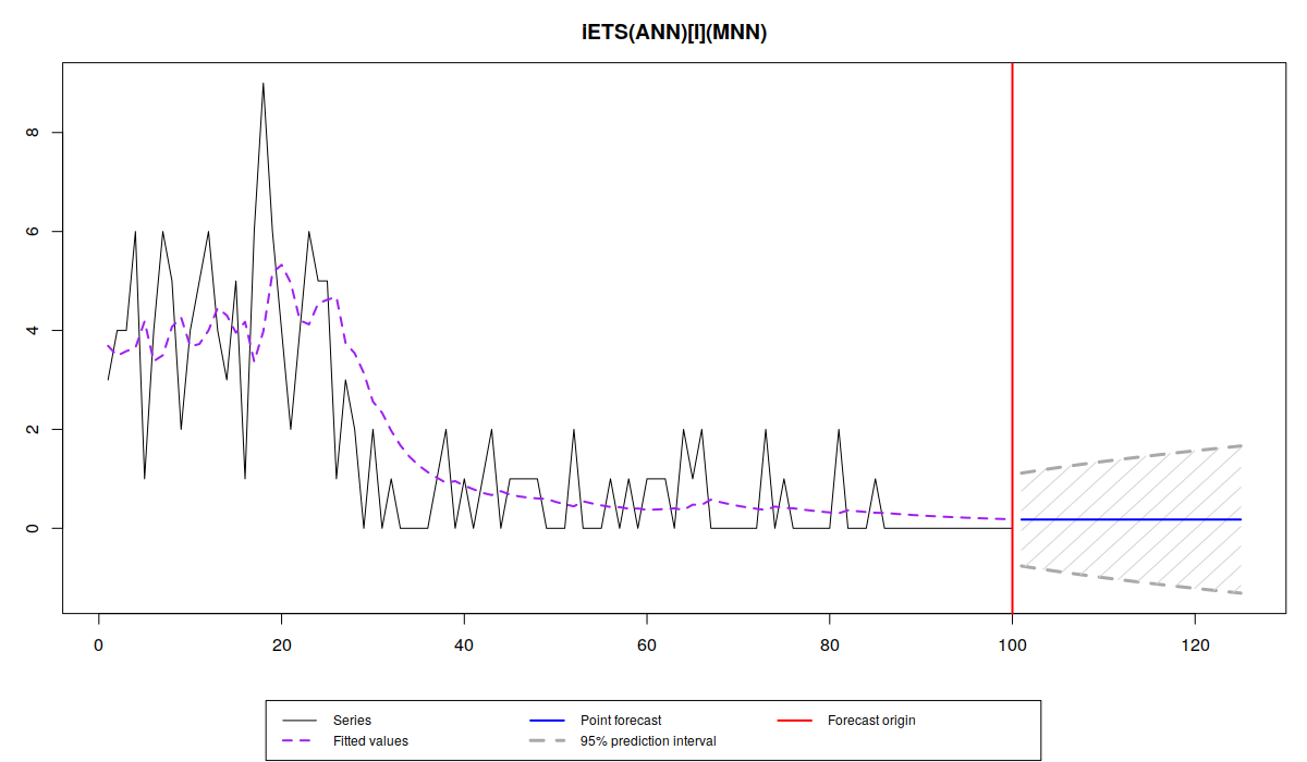
In the latter case the prediction intervals cover the negative part of the plane which does not make sense in our context. Note also that the information criteria are lower for the multiplicative model, which is due to the changing variance in sample for each 25 observations.
The important thing to note is that although multiplicative trend model sounds solid from the theoretical point of view (it cannot produce negative values), it might be dangerous in cases of small samples and positive trends. In this situation the model can produce exploding trajectory, because the forecast corresponds to the exponent. I don’t have any universal solution for this problem at the moment, but I would recommend using ETS(M,Md,N) (damped multiplicative trend) model instead of ETS(M,M,N). The reason why I don’t recommend ETS(M,A,N), is because in cases of negative trend, with the typically low level of intermittent demand, the updated level might become negative, thus making model inapplicable to the data.
As you see, there is now five new options for the models, which might complicate things in practice. Now we need to understand, how to select the most appropriate model for the demand occurrence between these five and how to make them more flexible, so that the trend and seasonal components are taken into account in demand occurrence, potentially together with some explanatory variables. If we can have a model that does all that, it would make it universal for a wide variety of data... One could only dream... right?
Interesting post! Can you elaborate on how one could tackle the problem of seasonal intermittency/absence, as with the watermelons only being sold for part of the year? I’m currently facing this issue with some products being sold only for 4-5 months per year,, where they have continuous demand, and then no demand at all for the remaining months.
I have thought about using a different frequency for the time series and removing the periods with no sales, but sadly the starting and ending period are not always in the same week each year.
Hi Casper,
I don’t have a specific model for that yet, and I have not covered some specifics of the functions of smooth in order to give the detailed answer. But if you know when the sales start and when they end (so you know specific values for o_t), then you can provide those values as a vector of dummies in the intermittent parameter. The other option would be to model time varying probability based on ETS(M,N,M) model for demand occurrence (meaning that there are periods, when probability is very high and the others, when it’s very low), but this relies on logistic model that has not been covered yet, and has its own limitations. I will discuss it in the next post.
Cheers,
Ivan
Hi Ivan,
Thanks for your answer. I do happen to know when the sales start and end, so I think the first approach would make most sense.
What do you mean exactly when you say to provide the dummy vector to the intermittent parameter? I tried fitting a model like this:
es(data, “MNN”, intermittent = dummy_vector, h = h), and got an error (i also tried fitting other types than MNN).
In general this thing that you use:
es(data, “MNN”, intermittent = dummy_vector, h = h)
should work. If it doesn’t then it’s possible that you found a bug. Can you, please, report it here: https://github.com/config-i1/smooth/issues – so we can figure out what’s happening?
I restarted my R session and now it works – I’m not sure what happened.
The results are, however, not as great as I had hoped. The main issue is that the data is seasonal, but I can only estimate a non-seasonal model due to too few non-zero values. I guess this is due to the fact that the underlying model tries to estimate seasonality for all of the year, and I only have data for around 14 weeks during the winter?
Do you have any ideas for how to proceed? I haven’t come across anything solving this problem yet, although I feel it should be quite a common problem in retailing.
This happens sometimes, I’m not sure why…
The problem with seasonal models on intermittent data is exactly what you say – very low number of observations. So the default univariate models will struggle with fitting anything meaningful with seasonality. John Boylan, Stephan Kolassa and I are currently working on one of the potential solutions for this problem (using vector models instead of univariate ones), but this is an ongoing research, in an alpha stage…
One of the potential solutions for now is to use dummy variables for seasons instead (for the cases, where intermittent!=0) – this might work slightly better. You can use xreg parameter in es() for that. Please, let me know if this works.