


Today I want to tell you a story of naughty APEs and the quest for the holy grail in forecasting. The topic has already been known for a while in academia, but is widely ignored by practitioners. APE stands for Absolute Percentage Error and is one of the simplest error measures, which is supposed to show the accuracy of forecasting models. It has its sister PE (Percentage Error), which is as sinister as APE, but is supposed to give an information about the bias of forecasts (so we can see, if we systematically overforecast or underforecast). As for the quest for the holy grail, it is to find the most informative error measure, that does not have any flaws.
Let’s start with one of the most popular error measures, based on APE, that is very often used by practitioners and is called “MAPE” – Mean Absolute Percentage Error. It is calculated the following way:
\begin{equation} \label{eq:MAPE}
\text{MAPE} = \frac{1}{h} \sum_{j=1}^h \frac{|y_{t+j} -\hat{y}_{t+j}|}{y_{t+j}} ,
\end{equation}
where \(y_{t+j}\) is the actual value, \(\hat{y}_{t+j}\) is the forecasted value j-steps ahead and \(h\) is the forecasting horizon. This thing shows the accuracy of forecasts relative to actual values and it has one big flaw – its final value really depends on the actual value in the holdout sample. If, for instance, the actual value is very close to zero, then the MAPE will most probably be very high. Vice versa if the actual value was very high (e.g. 1m), then the resulting error will be very low.
Some people would say that it’s okay, and that there’s no problem at all. They would argue that MAPE was developed to show that, and in a way they will be right. But let us imagine the following situation with a company called “Precise consulting”. The company works in retail and sells different goods, and their sales manager Tom wants to have the most accurate forecasts possible. In order to stimulate forecasters to produce accurate forecasts, he has a tricky system. If a forecaster has MAPE less than 10%, then he gets a money bonus. Otherwise the forecaster is punished and Tom spanks him personally. Tom thinks that this is a good system, which stimulates forecasters to work better. As for the forecasters, there is a forecaster Siegfried, who always gets bonuses and Roy, who always gets spanked. The first mainly deals with time series of the following type:
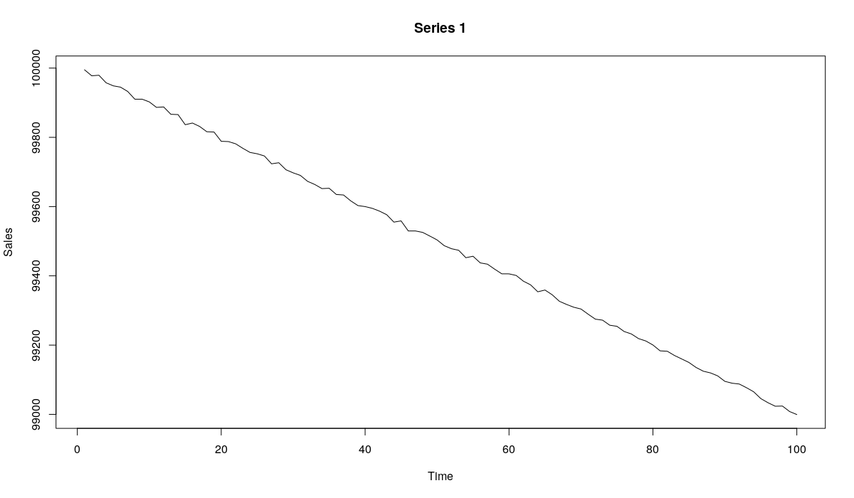
x1 <- 100000 - 10*c(1:100) + rnorm(100,0,5)
While the second has:
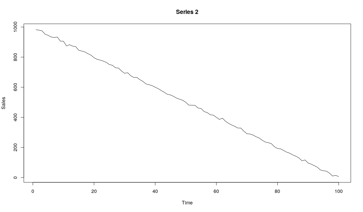
x2 <- 1000 - 10*c(1:100) + rnorm(100,0,5)
As you see, Siegfried has data with a level of sales close to 100k, while Roy has data with a level around 1k. They both don’t have appropriate education in forecasting, so although their data has trends, they both use simple exponential smoothing the following way:
es(x1,"ANN",silent=F,holdout=T,h=10)
es(x2,"ANN",silent=F,holdout=T,h=10)
The graphs in both cases look very similar:
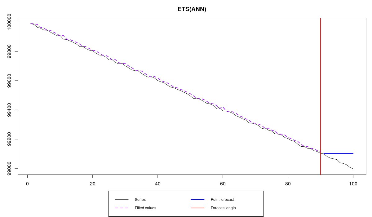
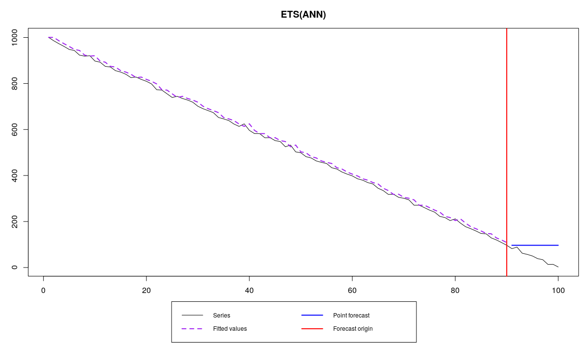
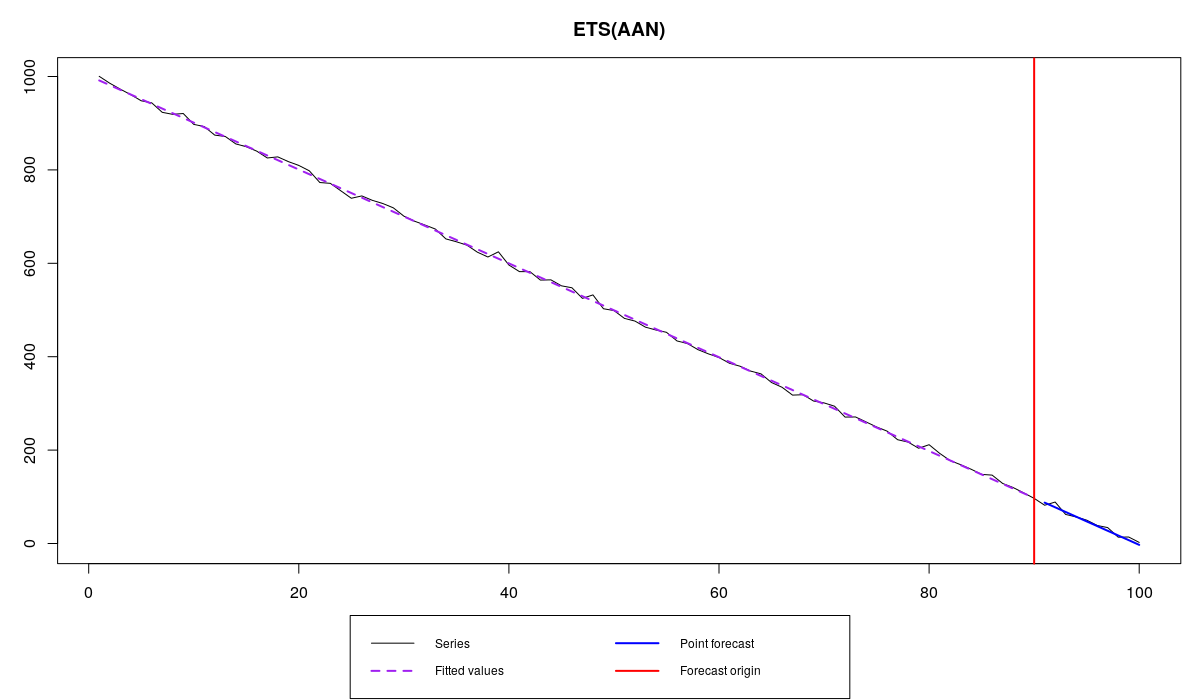
As we see, they both do lousy job as forecasters, not able to be precise. However Siegfried is a lucky guy, that’s why he has MAPE=0.1% and nice bonuses each month. Roy on the other hand is cursed with a bad time series and has MAPE=575.3%, so no bonuses for him. As you can see from the graphs above, the problem is not in Roy’s inability to produce accurate forecasts, but in the error measure that Tom makes both forecasters use. In fact, even if Roy uses the correct model (which would be ETS(A,A,N) or Holt’s model in this case), he would still get punished, because MAPE would still be above the threshold, being equal to 35.3%:
es(x2,"AAN",silent=F,holdout=T,h=10)
Roy is lucky enough not to have zeroes in the holdout sample. Otherwise he would have infinite MAPE and probably would get fired.
One would think that using Median APE could solve the problem, but it really doesn’t, because we still have the same levels’ influence on errors. And I’m not even mentioning the aggregation of MAPEs over several time series. If we do that, we won’t have anything meaningful and useful as well, because the errors on series with lower levels would overlap the errors on series with higher levels.
So, this is why APEs are naughty. Whenever you have error measure, where any value is divided by the actual value from the same sample, you will most likely encounter problems. MPE, mentioned above, has exactly the same problem. It is calculated similarly to MAPE, but without absolute values. In our example Siegfried has MPE=-0.1%, while Roy has MPE=-575.3% if he uses the wrong model and MPE=26.8% if he uses the correct one. So, this error measure does not provide the correct information about the forecasts as well.
Okay. So, now we know that using MAPE, APE, MPE and whatever else ending with PE is a bad idea, because it does not do what it is supposed to do and as a result does not allow making correct managerial decisions.
Tom, being a smart guy, and having read this post, decided to use a different error measure. He saw people mentioning in forecasting literature Symmetric MAPE (SMAPE):
\begin{equation} \label{eq:SMAPE}
\text{SMAPE} = \frac{2}{h} \sum_{j=1}^h \frac{|y_{t+j} -\hat{y}_{t+j}|}{|y_{t+j}| + |\hat{y}_{t+j}|} .
\end{equation}
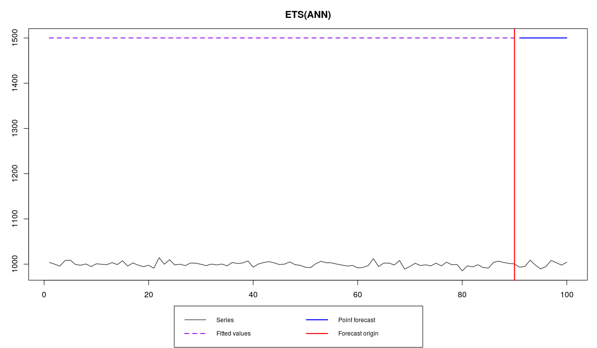
The idea of this error measure is to make it less biased by dividing the absolute value by the average of forecast and actual values (thus the appearance of 2 in the formula). Tom thinks that if this error measure is called “Symmetric”, then it should solve all of his problems. Now he asks Siegfried and Roy to report SMAPE instead of MAPE. And in order to test their forecasting skills, he gives both of them a very simple time series, with a fixed level (deterministic level):
x <- rnorm(100,1000,5)
Either out of fun or out of lack of knowledge Siegfried produced weird forecast, overshooting the data:
es(x,"ANN",silent=F,holdout=T,h=10,persistence=0,initial=1500)
while Roy did similar bad job, systematically underforecasting:
es(x,"ANN",silent=F,holdout=T,h=10,persistence=0,initial=500)
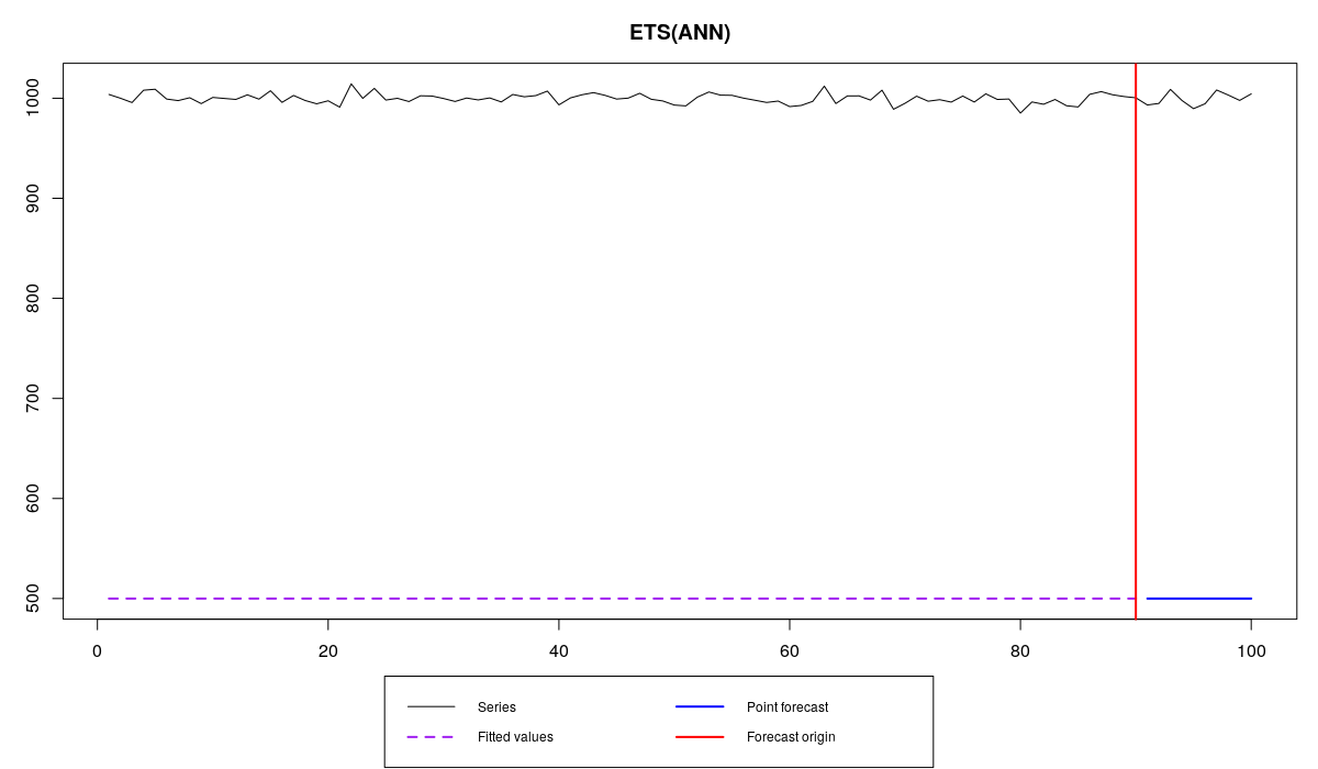
Obviously, both of them did similarly bad job, not getting to the point (and probably should be fired). But SMAPE would be able to tell that, right? You won’t believe it but it tells us that Siegfried still did a better job than Roy. He has SMAPE=40.1%, while Roy has SMAPE=66.6%. Judging by SMAPE alone, Tom would be inclined to fire Roy, although in reality he is as bad as Siegfried. What has happened? Are we missing something important in the performance of forecasters? Is Siegfried really doing a better job than Roy?
No! The problem is once again in the error measure - we are dealing with a naughty APE. This time we inflate the value of the error when the forecast is high, because of the inclusion of forecasts in the denominator of \eqref{eq:SMAPE}. This means that SMAPE likes, when we overforecast (this has been discussed in the literature first time by Goodwin and Lawton, 1999). Very bad APE! Very naughty APE! No one should EVER use it!
Okay. Now we know that there are bad APEs. What about good ones? Unfortunately, there are no good APEs, but there are other decent error measures.
Tom needs an error measure that would be applicable to a wide variety of data, would not have such dire problems and would be easy to interpret. As you probably already understand, there is no such thing, but at least there are better alternatives to APEs:
- sMAE – scaled Mean Absolute Error (proposed by Fotios Petropoulos and Nikos Kourentzes in 2015), which is also sometimes referred to as "weighted MAPE" or "wMAPE":
- MASE – Mean Absolute Scaled Error (proposed by Rob J. Hyndman and Anne B. Koehler in 2006)
- rMAE – Relative MAE (discussed in Andrey Davydenko and Robert Fildes in 2013)
\begin{equation} \label{eq:sMAE}
\text{sMAE} = \frac{\text{MAE}}{\bar{y}},
\end{equation}
where \(\bar{y}\) is average value of in-sample actuals and \(\text{MAE}=\frac{1}{h} \sum_{j=1}^h |y_{t+j} -\hat{y}_{t+j}|\) is Mean Absolute Error of the forecast for the holdout. This is a better analogue of MAPE, which is easy to interpret (it can also be measured in percentage). Unfortunately, it still has similar problems with different levels as MAPE has, but at least it does not react to potential zeroes in the holdout sample. Use it if you desperately need something meaningful, but at the same time better than MAPE.
\begin{equation} \label{eq:MASE}
\text{MASE} = \frac{\text{MAE}}{\frac{1}{t-1} \sum_{j=2}^t |y_{j} -y_{j-1}|}.
\end{equation}
The main thing of MASE is the division by the first differences of in-sample data. Sometimes the denominator is interpreted as an in-sample one-step-ahead Naive error. This thing allows bringing different time series to the same level and get rid of potential trend in the data, so you would not have that naughty effect of APEs. This is a more robust error measure than sMAE, it has fewer problems, but at the same time it is much harder to interpret than the other error measures. For example, MASE=0.554 does not really tell us anything specific. Yes, it seems that the forecast error is lower than the mean absolute difference of the data, but so what? This is a better error measure than any APE, but good luck explaining Tom what it means!
\begin{equation} \label{eq:rMAE}
\text{rMAE} = \frac{\text{MAE}_1}{\text{MAE}_2},
\end{equation}
here \(\text{MAE}_1\) is MAE of the model of interest, while \(\text{MAE}_2\) is MAE of some benchmark model. The simplest benchmark is Naive method. So by calculating rMAE we compare the performance of our model with Naive. If our model performs worse than the benchmark, then rMAE will be greater than one. If it is more accurate, then rMAE is less than one. In fact, rMAE aligns very well with so called "Forecast Value":
\begin{equation} \label{eq:FVA}
\text{FV} = (1-\text{rMAE}) \cdot 100\text{%} .
\end{equation}
So, for example, if rMAE=0.95, then we can conclude that the tested model is 5% better than the benchmark. This would be a perfect error measure, our holy grail, if not for a couple of small "Buts" – if for some reason \(\text{MAE}_2\) is equal to zero, rMAE cannot be estimated. Furthermore, it is recommended to aggregate rMAE over different time series using geometric mean rather than arithmetic one (because this is a relative error). So if on some time series the chosen model performs very well (e.g. MAE is very close to zero or even equal to zero), then rMAE will be close to zero as well, which will bring the aggregated value close to zero as well no matter what, even if in some cases the model did not perform well.
One more thing to note is that none of the discussed error measures can be applied to intermittent data (the data with randomly occurring zeroes). But this is a completely different story with completely different set of forecasters and managers.
As a conclusion, I would advise Tom not to use percentage error, but to use several other error measures, because each of them has some problems. Trying to find one best error measure is similar to the search for the holy grail. Don’t waste your time! And, please, don’t set bonuses or punishments for forecasters based on error measures – it’s a silly idea, which demotivates people to work well, but encourages them to cheat.