


While the previous posts on es() function contained two parts: theory of ETS and then the implementation – this post will cover only the latter. We won’t discuss anything new, we will mainly look into several parameters that the exponential smoothing function has and what they allow us to do.
We start with initialisation of es().
History of exponential smoothing counts dozens of methods of initialisation. Some of them are fine, some of them are very wrong. Some of those methods allow preserving data, the others unnecessarily consume parts of time series. I have implemented ETS in a way that allows initialising it before the sample starts. So the state vector \(v_t\) discussed in parts 2 and 3, is defined before the very first observation \(y_1\). This is consistent with Hyndman et al. (2008) approach. Still this initial value can be defined using different methods:
- Optimisation. This means that the initial value is found along with the smoothing parameters. This can be triggered by
initial="optimal"and is the default method ines(). - Backcasting. In order to define the initial value model is fitted to data several times going forward and backwards. For example, for ETS(A,N,N) the formula used for the forward is:
- Arbitrary values. If for some reason we know initial values (either from a previous data or from similar data), then we can provide them to
es(). In this case we may provide two parameters:initialandinitialSeason. The function will then use the provided values and fit the model. We can provide both of them or just one of them, meaning that the other will be estimated during the optimisation. Obviously if we deal with non-seasonal model, we don’t needinitialSeasonat all. A thing to note is that we cannot use backcasting when we define parameters manually. The other important thing to note is that the model selection and combinations do not work with predefined initial values, so this method of initialisation is not available when we need to select the best model or combine several forecasts usinges().
While the optimisation works perfectly fine on monthly data, there may be some problems with weekly and daily seasonal data. The reason for that is a high number of parameters that need to be estimated. For example, ETS(M,N,M) on weekly seasonal data will have 52 + 1 + 2 + 1 = 56 parameters to estimate (52 seasonal indices, 1 level component, 2 smoothing parameters and 1 variance of residuals). This is not an easy task which sometimes cannot be efficiently solved. That is why we may need other initialisation methods.
Let’s see what happens when we encounter this problem in an example. I will use time series taylor from forecast package. This is half-hourly electricity demand data. It has frequency of 336 (7 days * 48 half-hours) and is really hard to work with when the standard initialisation is used. Let’s see what happens when es() is applied with model selection and a holdout of one week of data:
es(taylor,"ZZZ",h=336,holdout=TRUE)
Forming the pool of models based on... ANN, ANA, ANM, AAA, Estimation progress: 100%... Done!
Time elapsed: 18.47 seconds
Model estimated: ETS(ANA)
Persistence vector g:
alpha gamma
0.850 0.001
Initial values were optimised.
340 parameters were estimated in the process
Residuals standard deviation: 250.546
Cost function type: MSE; Cost function value: 56999

Information criteria:
     AIC     AICc      BIC
51642.90 51712.02 53756.01
Forecast errors:
MPE: 1%; Bias: 50%; MAPE: 1.8%; SMAPE: 1.8%
MASE: 0.798; sMAE: 1.8%; RelMAE: 0.078; sMSE: 0.1%
We had to estimate 340 parameters and the model selection took 18 seconds (checking only 5 models in the pool). We ended up with the following graph:
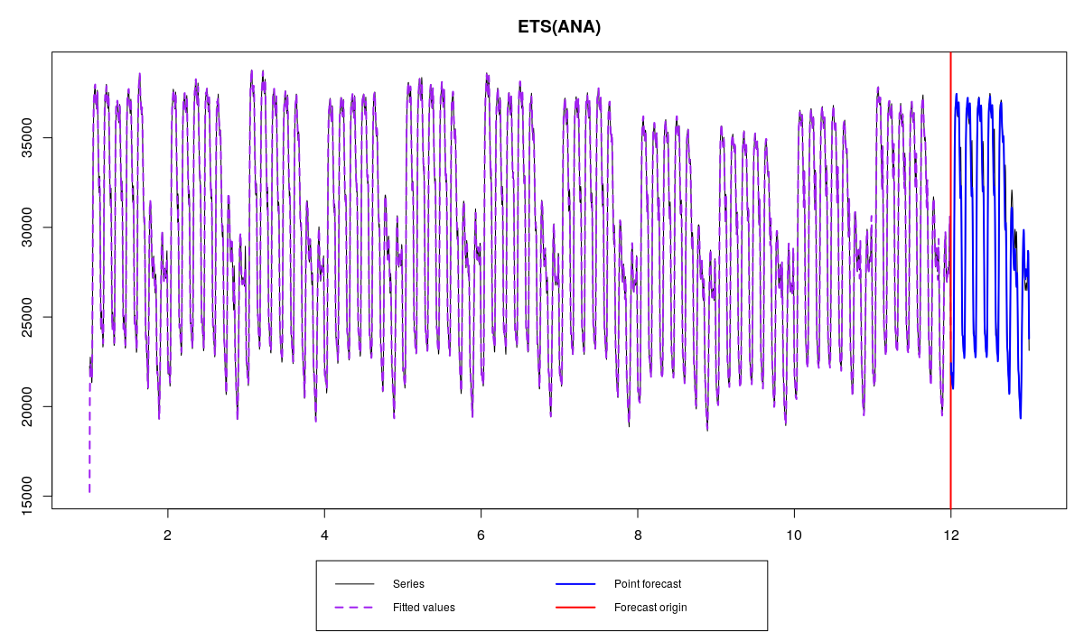
Electricity demand series with ETS(A,N,A) initialised using optimisation and its forecast
The first thing that can be noticed is the initial value of level, which results in a wrong one step ahead forecast for one of the first observations. This is because of the high number of parameters – the optimiser could not find the appropriate values. This could be not important, taking number of observations in the data, but still may influence the final forecast and, what is more important, the model selection. Some of models could have been initialised slightly better than the others, which could lead to a smaller value of information criterion for those models that should not have been selected.
This example motivates the other initialisation mechanisms.
\begin{equation} \label{eq:ETSANN_Forward}
\begin{matrix}
y_t = l_{t-1} + \epsilon_t \\
l_t = l_{t-1} + \alpha \epsilon_t
\end{matrix}
\end{equation}
while for the backwards it should be changed to:
\begin{equation} \label{eq:ETSANN_Backward}
\begin{matrix}
y_t = l_{t+1} + \epsilon_t \\
l_t = l_{t+1} + \alpha \epsilon_t
\end{matrix}
\end{equation}
As you see, the only thing that changes is the lower index of level component. The formula \eqref{eq:ETSANN_Forward} is used for fitting of the model to the data starting from the first observation till the end of series. When we reach the end of series, we use formula \eqref{eq:ETSANN_Backward} and move from the last observation to the very first one. Then we produce forecast back in time before the initial \(y_1\) and obtain the initial values for the components. The model is then fit to the data using these initials. This procedure can be repeated several times in order to get more accurate estimates of the initial values. In es() it is done 3 times and can be triggered by initial="backcasting". As mentioned above this method of initialisation is recommended for data with high seasonality frequencies (weekly, daily, hourly etc).
As an example, we will use the same time series from forecast package:
es(taylor,"ZZZ",h=336,holdout=TRUE,initial="b")
This time all the process takes around 7 seconds:
Forming the pool of models based on... ANN, ANA, ANM, AAA, Estimation progress: 100%... Done!
Time elapsed: 6.81 seconds
Model estimated: ETS(MNA)
Persistence vector g:
alpha gamma
    1     0
Initial values were produced using backcasting.
3 parameters were estimated in the process
Residuals standard deviation: 0.007
Cost function type: MSE; Cost function value: 38238

Information criteria:
     AIC     AICc      BIC
49493.46 49493.47 49512.11
Forecast errors:
MPE: 0.8%; Bias: 40.6%; MAPE: 1.7%; SMAPE: 1.8%
MASE: 0.784; sMAE: 1.7%; RelMAE: 0.076; sMSE: 0.1%
The function has checked the same pool of models and selected ETS(M,N,A) as the optimal model (estimating only 3 parameters). We ended up with a peculiar model, where smoothing parameter for the level is equal to one (meaning that we have random walk in the level) and the other parameter equal to zero (meaning that we have deterministic seasonality).
The graph of the model now looks reasonable:
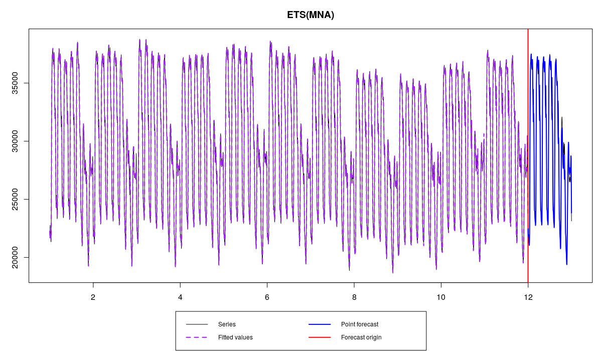
Electricity demand series with ETS(M,N,A) initialised using backcasting and its forecast
As it can be seen from the Figure, backcasting is not a bad technique and it can be useful in cases when we have a data with high frequencies. Furthermore, there is a proof that backcasting asymptotically gives the same estimates as least squares, meaning that both optimal and backcasted estimates of initial values should eventually converge to the same values.
Continuing our example, we will use classical decomposition and construct ETS(M,N,M) model
ourFigure <- decompose(taylor,type="m")$figure
es(taylor,"MNM",h=336,holdout=TRUE,initial=mean(taylor),initialSeason=ourFigure)
Time elapsed: 3.97 seconds
Model estimated: ETS(MNM)
Persistence vector g:
alpha gamma
    1     0
Initial values were provided by user.
340 parameters were estimated in the process
Residuals standard deviation: 0.007
Cost function type: MSE; Cost function value: 37783

Information criteria:
     AIC     AICc      BIC
50123.24 50192.36 52236.34
Forecast errors:
MPE: 0.7%; Bias: 35%; MAPE: 1.6%; SMAPE: 1.7%
MASE: 0.738; sMAE: 1.6%; RelMAE: 0.072; sMSE: 0.1%
We can even compare results of this call with other initialisation methods:
es(taylor,"MNM",h=336,holdout=TRUE,initial="o")
Time elapsed: 13.13 seconds
Model estimated: ETS(MNM)
Persistence vector g:
alpha gamma
0.919 0.000
Initial values were optimised.
340 parameters were estimated in the process
Residuals standard deviation: 0.009
Cost function type: MSE; Cost function value: 56381

Information criteria:
     AIC     AICc      BIC
51602.59 51671.70 53715.69
Forecast errors:
MPE: 0.9%; Bias: 40.6%; MAPE: 1.8%; SMAPE: 1.8%
MASE: 0.791; sMAE: 1.7%; RelMAE: 0.077; sMSE: 0.1%
es(taylor,"MNM",h=336,holdout=TRUE,initial="b")
Time elapsed: 6.52 seconds
Model estimated: ETS(MNM)
Persistence vector g:
alpha gamma
    1     0
Initial values were produced using backcasting.
3 parameters were estimated in the process
Residuals standard deviation: 0.007
Cost function type: MSE; Cost function value: 37272

Information criteria:
     AIC     AICc      BIC
49398.88 49398.89 49417.52
Forecast errors:
MPE: 0.8%; Bias: 33.8%; MAPE: 1.7%; SMAPE: 1.8%
MASE: 0.786; sMAE: 1.7%; RelMAE: 0.076; sMSE: 0.1%
Estimation in this case takes approximately four seconds (on my PC), while for initial="o" it takes around 13 seconds and for initial="b" - near seven seconds. The resulting models in these cases look very similar, with the first model producing slightly more accurate forecasts.
This method of initialisation may be used when the other two methods for some reason do not work as expected (for example, take too much computational time) and/ or when we know the values from some reliable sources (for example, from previously fitted model to the same or similar data). It can also be used for fun and experiments with ETS. In all the other cases I would not recommend using it.
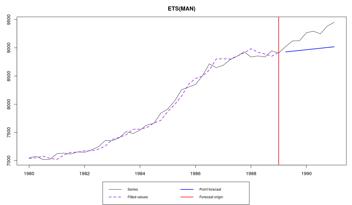
There are other exciting parameters in es() that can be controlled. They allow to switch between optimised and predefined values. For example, parameter persistence accepts vector of smoothing parameters, the length of which should correspond to the number of components in the model, while parameter phi defines damping parameter. So, for example, ETS(A,Ad,N) fitted to a time series N1234 from M3 can be constructed using:
es(M3$N1234$x,"AAdN",h=8,persistence=c(0.2,0.1),phi=0.95)
Compare the resulting graph:
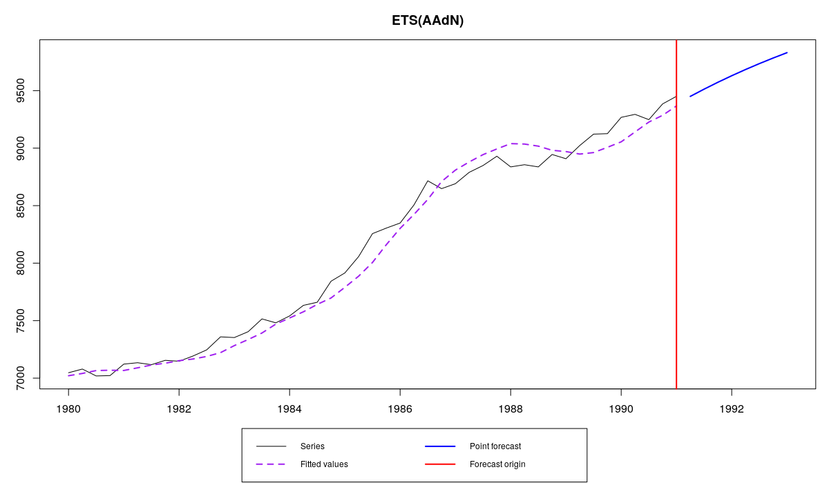
Series N1234 and ETS(A,Ad,N) fit to it with predefined parameters
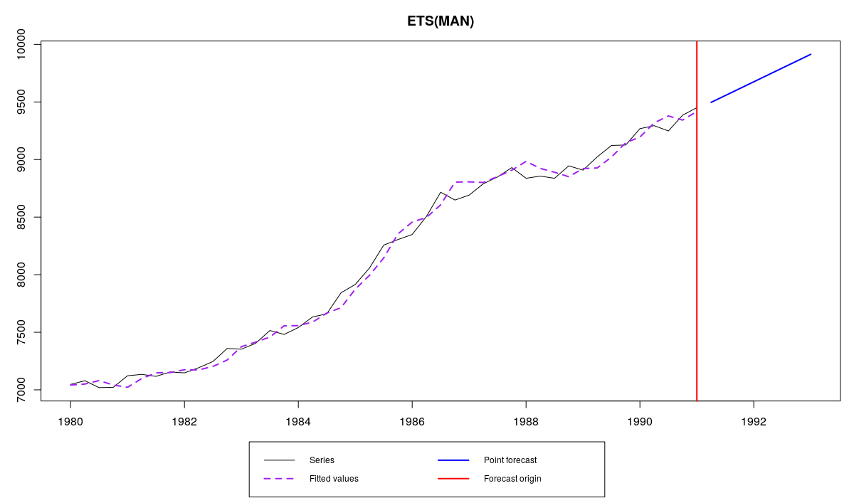
with the one from optimised model:
es(M3$N1234$x,"AAdN",h=8)
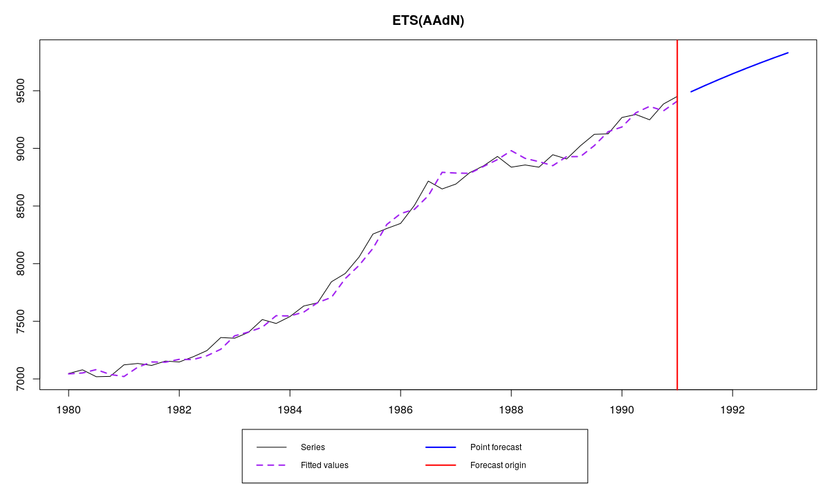
Series N1234 and ETS(A,Ad,N) fit to it with optimised parameters
I cannot say which of them is better in means of accuracy, but if you really need to define those parameters manually (for example, when applying one and the same model to a large set of time series), then you can easily do it, and now you know how.
One other cool thing about es() is that it saves all the discussed above values and returns them as a list. So you can save a model and then reuse the parameters. For example, let’s select the best model and save it:
ourModel <- es(M3$N1234$x,"ZZZ",h=8,holdout=TRUE)
Which gives us:
Series N1234 and ETS(M,A,N) fit to it with optimised parameters
Now we will use a small but neat function called modelType(), which extracts type of model, and use exactly the same model with exactly the same parameters but with a larger sample:
es(M3$N1234$x,modelType(ourModel),h=8,holdout=FALSE,initial=ourModel$initial,persistence=ourModel$persistence,phi=ourModel$phi)
This now results in the same model but with the updated states, taking into account the last ушпре observations:
Series N1234 and the same ETS(M,A,N) fit to a larger sample
The other way to do exactly the same is just to pass ourModel to es() function this way:
es(M3$N1234$x,model=ourModel,h=8,holdout=FALSE)
This way we can, for example, do rolling origin with fixed parameters.
The function modelType() also works with models estimated using ets() function from forecast package, so you can easily use ets() and then construct the model of the same type using es():
etsModel <- ets(M3$N1234$x)
es(M3$N1234$x,model=modelType(etsModel),h=8,holdout=TRUE)
Not sure why you would need it, but here it is. Enjoy!
That’s it for today. I hope that this post was helpful and now you know what you can do when you don’t have anything to do. See you next time!