All the examples on this website use R. So it is reasonable to come up with a brief tutorial on how to install it and use it.

R for Windows can be downloaded from here. It is recommended to install it in a root folder, something like “C:\R\” – there have been reports of some issues over the years, when the program is installed in difficult folders, such as “Program files”. However, you might not encounter those problems, but you never know…

As for Mac, the program can be downloaded from here.

Finally, R for Linux is usually available from the default repository. I use Debian-based systems, so the standard command in terminal for installing R is:

sudo apt-get install r-base

Working with core R only is something that only advanced users can do – not many people would agree to use pure command line and not be able to see the graphs and tables in the same window. So, there are front ends for R, the most popular of which is RStudio, which can be downloaded from here. It brings all the necessary elements in one interface, simplifying the whole analysis and forecasting process.

From now on we assume that you have managed to install both R and RStudio. So, let’s see what we have got.

The interface of RStudio

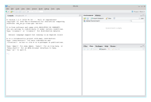
Here’s the default view of the interface of RStudio:

R works with projects. Project is just a collection of tables, arrays, variables, scripts. Whenever you close a project, all its environment is automatically saved, so that you can always come back to it and continue your work. The name of the project is shown in the top right corner of RStudio (by default it is “None”). If you click on that name and select “New project”, then you will be greeted with a dialogue, proposing to create a new project. Then there are several options for the project, but for the acquaintance with R it is sufficient to select “New Directory”, “Empty Project” and then select the folder for the project on your drive and enter project’s name. Why not start a project called “Open Forecast”? Having several project for different purposes, it is very easy to switch between them, continuing the work that you have started some time ago and saving the progress.

The left part of the screen contains the command line. This is the main instrument of R. You will type your commands there and see the results. For example, let’s type this:

x <- rnorm(100,0,1)

This command generates a vector of 100 random numbers from standard normal distribution and then writes it to the object called "x". The symbol "<-" is equivalent to "=" and shows what values to assign to the object on the left hand side. Sometimes it might be easier to use a different symbol: "->", which works identically to the previous one, but assigning the value from left to right. For example, this way we create a variable "y" that contains exactly the same values as the variable "x":

x -> y

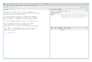
You might have already noticed, that these variables have appeared in the so called "Environment", in the top right part of the screen:

This tab contains all the objects that we save in the project. For example, if we create the following matrix:

\( A = \begin{pmatrix} 1 & 1 \\ 0 & 1 \end{pmatrix} \)

with this command:

A <- matrix(c(1,0,1,1),2,2)

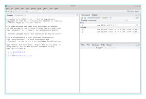
then it will appear in the «Environment» tab:

Now that we are more or less familiar with the interface of RStudio, let's have a look at the R functions.

Any function that we use needs some parameters. For example, the function matrix() needs the following parameters:

• data – either vector or a matrix that contains some values;
• nrow – number of rows;
• ncol – number of columns;
• byrow — logical parameter, telling how to allocate the data in the matrix. If "TRUE", then the matrix will be filled in from left to right, row by row. Otherwise it will fill in the matrix from top to bottom column by column. The default value is "FALSE";
• dimnames — a list of names for rows and columns.

Some of these parameters have default values (e.g. byrow=FALSE), while the others can be omitted (e.g. dimnames), and the rest must be provided by user (e.g. data).

One of the features of R is that the values can be passed to any function either directly specifying the parameter and its value, or sequentially. So the following two commands are equivalent, because we know the sequence of the parameters in the function:

A <- matrix(data=c(1,0,1,1), nrow=2, ncol=2)
A <- matrix(c(1,0,1,1), 2, 2)

If we need to specify a parameter, skipping some steps in the sequence, then we need to call it explicitly:

A <- matrix(c(1,0,1,1), 2, 2, dimnames=list(c("A","B"),c("C","D"))

If you forget at any point in time what parameters the function accepts, you can always ask for help the following way:

?matrix

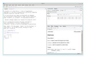
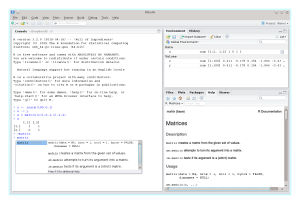
here "matrix" is the name of the function of interest. RStudio will open a tab «Help» for you with the description of the function:

You can also use the "Search" on the "Help" tab in order to find the function of interest.

As a small trick, if you don't remember the full name of a function or a variable, you can start typing its first letters and press "Tab". RStudio will show you the relevant objects:

Now that we have created some variables, we can look at them. The easiest way to do that is to print its name in the command line:

A

The other option is to press on the name of the variable in the Environment tab. If you want to work with the matrix or a table in a style similar to Excel, then there are functions "View" and "edit" that might help:

View(A)
edit(A)

Note that R is case sensitive, so "View" is not the same as "view".

Okay. So, we are more or less comfortable with the interface and some basic objects and functions. Even though the command line is the main area in RStudio, it's not always nice to retype things over and over again. So you can either select the "History" tab in the top right corner and find the command that you need, or you can press buttons "Up" and "Down" in the command line in order to select the previous command. Another alternative is to press "Ctrl+Up", which will show the list of several last commands.

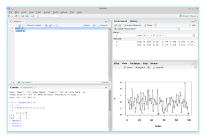
However, sometimes, you need something more flexible than just History, something that can be reproduced in different projects. And here come scripts. You can create one by pressing "plus" sign in the top left corner and selecting "R Sctipt". In the newly opened tab, you can write functions, comments, calls to variables and so on. For example, if we want to construct a linear graph of "x" with points, we can do type the following in the script window:

plot(x)
lines(x)

The first function will construct a simple point graph, and the second will add lines over them, connecting them sequentially. If you select these two commands in the script and press "Ctrl+Enter", then they will be executed one after another. As a result RStudio will open a new tab, "Plot" in the bottom right area and will demonstrate the graph:

If you want to reuse the script at any point in future, you can save it ("Save" icon in the top left side of the screen).

By the way, RStudio contains a lot of useful shortcuts, which substantially simplify the work with the program. Have a look here.

Packages

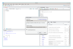
As it is discussed in another section of the website, there is a plethora of packages for R. The majority of them are located on CRAN repository and can be easily installed from RStudio. All you need to know is the name of the package. The installation and the update of packages can be done via the "Packages" tab in the bottom right area. There you can click "Install" button in order to see the following:

Let's install one of the packages, called "smooth", maintained by the CMAF members by typing its name in the new window. Press "Install" after that and RStudio will download the package, all the necessary dependencies and install all of that to your computer. As an alternative, you can install packages from the command line by typing:

install.packages("smooth")

In order to use the installed package, it needs to be attached to the environment using the command:

library(forecast)

As an alternative, you can find the name of the package on the "Packages" tab and tick the box on the left side of the name.

After the load of the package, all its functions will become available. For example, here's an sma() function from "smooth" package, which constructs simple moving averages in state-space form:

sma(x, silent=FALSE)

This will select the appropriate order of SMA and fit the model to the data.

Very often we will work with the specific type of object in R, which is called "ts" - time series. In order to transform a variable from a vector to ts, we need to run:

x <- ts(x,start=c(1984,1),frequency=12)

where "start" is the parameter, setting the starting point for the time series (in our example it is January 1984) and "frequency" is the periodicity of the data. So, for example if we work with monthly data, frequency=12, and in case of quarterly it will be equal to 4. After using this command, the object x will be transformed from vector to ts. Some functions in R will now work slightly differently. For example, try plotting "x" in order to see if the result is different from what we have previously done.

These are the main elements of R and RStudio that we need in order to proceed with more advanced tutorials. If you want to learn more, there are courses on Coursera and on DataCamp, that might be helpful.

Additional tasks

And here are some tasks. Type the following lines of code (one by one) and see what you get in return. This way you will familiarise yourself with R:

(41/3 + 78/4)*2
2^3+4
1/0
0/0
max(1,min(-2,5),max(2,pi))
sqrt(3^2+4^2)
exp(2)+3i
log(1024)
log(1024, base=2)
c(1:3)
c(1:5)*2 + 4
x <- 10 + c(1:10)*0.5 + rnorm(10,0,2)
x
mean(x)
var(x)
x <- ts(x,start=c(2010,2),frequency=4)