


Over the year 2017 the smooth package has grown from v1.6.0 to v2.3.1. Now it is much more mature and has more downloads. It even now has its own hex (thanks to Fotios Petropoulos):

A lot of changes happened in 2017, and it is hard to mention all of them, but the major ones are:
- Introduction of ves() function (Vector Exponential Smoothing);
- Decrease of computation time of es(), ssarima() and other functions;
- More flexibility in es() function;
- Development of model selection mechanism for exogenous variables (this will be covered in one of the next posts in a couple of weeks);
- Development of intermittent data model for es(), ssarima(), ces() and ges() (will also be covered in one of the posts in 2018);
- Introduction of auto.ges() function, which allows selecting the most appropriate GES model for the data (once again, a post on that is planned);
- Switch to roxygen2 package for the maintenance purposes, which simplified my life substantially.
Not all of these things sound exciting, but any house is built brick by brick and some of those bricks are pretty fundamental. Now the new year has started, and I don’t have any intentions of stopping the development of smooth package. The 2018 will bring more interesting things and features, mainly driven by my research in multivariate models. At the moment I have the following list of features to implement:
- Intermittent VES model. This is driven by one of the topics I’m working together with John Boylan and Stephan Kolassa;
- Exogenous variables in VES model (also connected with that topic);
- Model selection mechanism in ves() models;
- Conditional intervals for VES model (currently only the version with independent intervals is implemented);
- State-space VARMA, which is needed for my research with Victoria Grigorieva and Yana Salihova;
- sim.iss() function, which should allow generating the occurrence part of intermittent data. This should be helpful for another research I plan to conduct together with John Boylan and Patricia Ramos;
- Vector SMA – the idea proposed by Mikhail Artukhov, this is yet another research topic;
- …And a lot of other cool things and features.
But before starting the work in those areas, I’ve decided to measure the performance of the most recent smooth functions (accuracy and computation time) and report it here. I used ets() and auto.arima() functions from forecast package as benchmarks. I have done this experiment in serial and included the following models:
- ES – the default exponential smoothing, ETS(Z,Z,Z) model produced by es() function from smooth;
- ESa – the same ETS model, but without multiplicative trends. This was needed in order to make a proper comparison with ets() function, which neglects the multiplicative trends by default. The call for this model is es(datasets[[i]],”ZXZ”). I report two versions of this thing: one from smooth v2.3.0 from CRAN and the other from smooth v2.3.1 available on GitHub. The latter has the advanced branch and bound mechanism for these types of models, while the former uses the brute force in model selection;
- SSARIMA – State-space ARIMA implemented in auto.ssarima() function from smooth;
- CES – Complex Exponential Smoothing via auto.ces() function from smooth;
- GES – Generalised Exponential Smoothing via auto.ges() function from smooth
- ETS – ETS model implemented in ets() function from forecast package;
- ETSm – ETS model with multiplicative trends, done via ets(dataset[[i]]$x, allow.multiplicative.trend=TRUE). This makes the function comparable with the default es();
- ARIMA – ARIMA model constructed using auto.arima() fucntion.
I used five error measures, some of which were discussed in the post about APEs, and aggregated them over the dataset using mean and median values. Here’s the list:
- MASE – Mean Absolute Scaled Error;
- sMAE – scaled Mean Absolute Error;
- RelMAE – Relative Mean Absolute Error (the benchmark in this case is a simple Naive and it should be aggregated using geometric mean rather than arithmetic);
- sMSE – scaled Mean Squared Error (MSE divided by the squared average actuals in-sample);
- sCE – scaled Cumulative Error (just the sum of errors divided by the average actuals in-sample);
The following code was used in the experiment, so feel free to use it for whatever purposes:
All the smooth functions can be applied to the data of class "Mcomp" directly: the in-sample data will be used for the fit of the model, the forecast of the needed length will be produced and then the accuracy of the forecast will be measured - everything in one go. Applying forecast functions is slightly trickier, and in order to have the same measurements I used Accuracy() function from smooth v2.3.1 (it is unavailable in earlier versions of the package).
I ended up having 5315 forecasts and I calculated those error measures for the whole dataset and for each of the following categories: yearly, quarterly, monthly and other data. You can find 6 tables with the results at the end of this page (the best value is in green bold). Things to notice are:
- ES performs similar to ETS, when they go through the similar models. e.g. ESa sometimes outperforms ETS and vice versa, but the difference is usually not significant (see, for example, Table 1. But this can also be observed in the other tables);
- ETS with multiplicative trends performs worse than the one without them. This holds for both es() and ets();
- SSARIMA performs (in terms of accuracy) similar to ARIMA on monthly and quarterly data, but fails on yearly data;
- CES and GES sometimes outperform other models, but this is not consistent;
- Branch and bound mechanism of es() is efficient and improves the performance of the function several times (29 minutes for the calculation of ESa v2.3.1 on the whole dataset vs 91 minutes of ESa v2.3.0) - see Table 6 for the details;
- The three fastest functions in the comparison are: ets() with the default parameters values, es() without multiplicative trends and ces()
Finally, I've conducted Nemenyi test using nemenyi() function from TStools package for RelMAE and for the computation time on the whole dataset in order to see if the differences between the models are on average statistically significant and how they rank (sort of average temperature in the hospital metrics). Keep in mind that this test compares the ranks of the contestants, but does not measure the distances between them. Here are the graphs produced by the function:
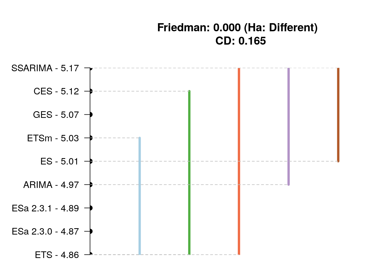
Overall accuracy of models
The graph above tells us that ETS, ES, ESa, ARIMA and ETSm overall perform similar to each other - they are in one group of models. The other models also perform very close to these, but probably slightly less accurate. In order to see if the difference between the models is indeed significant, we would need to conduct the similar experiment on a larger dataset (M4 maybe?).
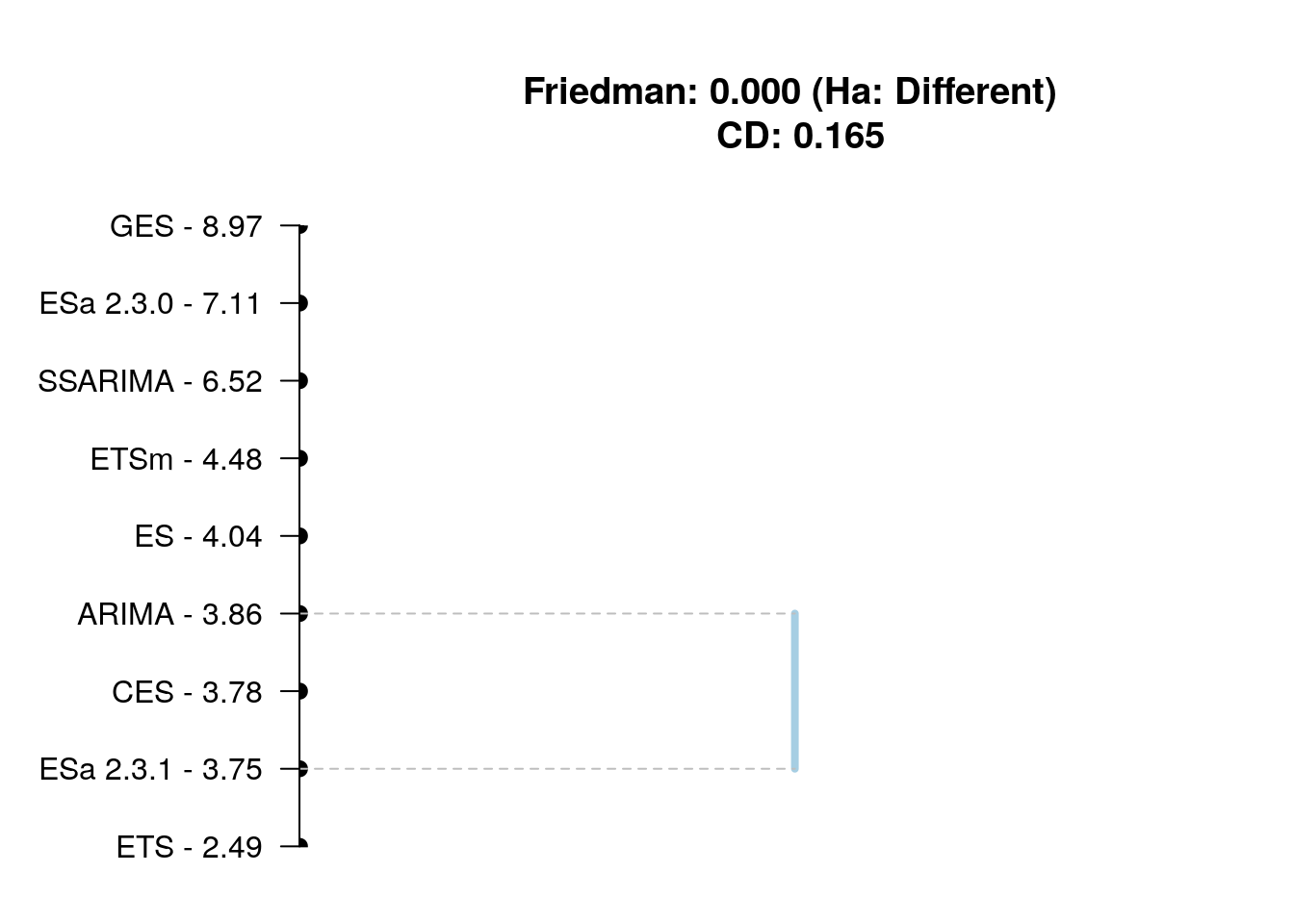
Computation time ranking
This graph tells us that ets() is significantly faster than all the other functions and that ESa, ES and ARIMA have similar performance. Once again, thing to keep in mind is that 0.0001 second is faster than 0.0002 seconds, which means that the former would have rank 1 and the latter would have rank 2. This explains, why ESa is overall faster than ETS (see Table 6), but the Nemenyi test tells us the opposite.
Concluding this New Year experiment, I would say that smooth package is a good package and can now be efficiently used for automatic forecasting. But I'm biased, so don't believe my words and give it a try yourselves ;).
Happy New Year!
| Mean | Median | |||||||||
| MASE | sMAE | RelMAE | sMSE | sCE | MASE | sMAE | RelMAE | sMSE | sCE | |
| ES | 236.8 | 25.7 | 74.7 | 167.2 | -9.9 | 136.2 | 13.2 | 89.1 | 2.5 | -12.9 |
| ESa | 224.8 | 23.4 | 73.4 | 30.0 | -37.3 | 133.4 | 12.9 | 88.0 | 2.4 | -17.2 |
| SSARIMA | 235.9 | 25.2 | 76.2 | 46.7 | -15.0 | 136.2 | 13.4 | 84.7 | 2.6 | -7.7 |
| CES | 233.7 | 25.5 | 75.5 | 52.8 | 8.4 | 136.7 | 13.5 | 81.3 | 2.6 | 2.1 |
| GES | 244.1 | 27.6 | 75.8 | 95.3 | 38.7 | 135.2 | 13.3 | 79.9 | 2.6 | 2.2 |
| ETS | 227.0 | 23.2 | 73.2 | 28.7 | -28.3 | 131.2 | 12.8 | 85.2 | 2.3 | -13.3 |
| ETSm | 241.6 | 25.9 | 75.0 | 53.8 | 8.9 | 133.7 | 13.1 | 85.8 | 2.5 | -8.7 |
| ARIMA | 232.6 | 24.7 | 74.6 | 38.2 | -11.2 | 132.5 | 13.3 | 82.4 | 2.5 | -7.4 |
| Mean | Median | |||||||||
| MASE | sMAE | RelMAE | sMSE | sCE | MASE | sMAE | RelMAE | sMSE | sCE | |
| ES | 332.4 | 45.1 | 89.9 | 598.9 | 25.2 | 211.1 | 21.2 | 100.0 | 5.8 | -17.0 |
| ESa | 300.7 | 37.7 | 86.2 | 78.1 | -34.6 | 206.9 | 20.4 | 100.0 | 5.4 | -25.2 |
| SSARIMA | 327.6 | 42.8 | 90.9 | 141.9 | -1.0 | 214.1 | 21.0 | 100.0 | 5.9 | -23.2 |
| CES | 323.3 | 43.8 | 89.2 | 163.3 | 45.5 | 203.5 | 19.8 | 94.0 | 4.9 | 2.1 |
| GES | 346.2 | 50.4 | 90.2 | 325.3 | 90.5 | 208.1 | 20.0 | 91.8 | 5.3 | 0.2 |
| ETS | 304.3 | 37.7 | 87.2 | 74.7 | -47.1 | 210.8 | 20.8 | 100.0 | 5.9 | -26.6 |
| ETSm | 340.0 | 45.3 | 91.7 | 150.4 | 18.9 | 216.2 | 21.4 | 100.0 | 6.2 | -16.9 |
| ARIMA | 312.1 | 41.0 | 86.9 | 107.7 | -5.7 | 207.6 | 20.8 | 100.0 | 5.7 | -20.4 |
| Mean | Median | |||||||||
| MASE | sMAE | RelMAE | sMSE | sCE | MASE | sMAE | RelMAE | sMSE | sCE | |
| ES | 211.2 | 20.2 | 70.9 | 18.6 | -27.7 | 129.8 | 11.4 | 80.4 | 1.8 | -10.9 |
| ESa | 202.6 | 19.6 | 69.6 | 14.5 | -44.0 | 128.3 | 10.8 | 78.8 | 1.6 | -15.4 |
| SSARIMA | 209.2 | 20.3 | 71.5 | 15.8 | -37.9 | 133.0 | 11.7 | 82.0 | 2.0 | -7.8 |
| CES | 209.8 | 19.7 | 71.0 | 14.1 | -7.1 | 127.4 | 11.9 | 77.0 | 1.9 | 4.4 |
| GES | 213.9 | 20.9 | 70.7 | 18.3 | 2.2 | 126.2 | 11.9 | 76.0 | 2.0 | 4.7 |
| ETS | 207.3 | 19.3 | 68.3 | 14.1 | -36.9 | 121.3 | 10.4 | 77.4 | 1.5 | -11.6 |
| ETSm | 214.9 | 20.0 | 69.9 | 14.9 | -18.1 | 126.7 | 11.3 | 78.1 | 1.7 | -6.4 |
| ARIMA | 209.2 | 20.2 | 69.7 | 15.7 | -23.3 | 124.3 | 11.5 | 77.6 | 1.8 | -3.5 |
| Mean | Median | |||||||||
| MASE | sMAE | RelMAE | sMSE | sCE | MASE | sMAE | RelMAE | sMSE | sCE | |
| ES | 202.2 | 19.6 | 70.9 | 23.9 | -20.5 | 106.2 | 12.1 | 79.5 | 2.2 | -19.0 |
| ESa | 198.3 | 18.9 | 70.4 | 14.2 | -38.3 | 105.5 | 12.1 | 78.3 | 2.1 | -21.4 |
| SSARIMA | 203.3 | 19.8 | 72.9 | 14.8 | -11.5 | 110.6 | 12.7 | 78.9 | 2.3 | -1.6 |
| CES | 199.0 | 20.1 | 72.1 | 17.1 | -3.6 | 112.3 | 12.7 | 78.1 | 2.4 | -3.6 |
| GES | 207.4 | 20.4 | 72.6 | 18.2 | 32.6 | 111.4 | 12.6 | 76.4 | 2.3 | -2.1 |
| ETS | 198.4 | 18.8 | 70.3 | 13.5 | -15.4 | 105.8 | 12.0 | 76.8 | 2.2 | -11.3 |
| ETSm | 206.4 | 20.0 | 71.2 | 26.2 | 18.9 | 106.6 | 12.1 | 77.8 | 2.2 | -9.8 |
| ARIMA | 205.4 | 19.7 | 72.8 | 15.2 | -8.6 | 111.0 | 12.5 | 78.3 | 2.3 | -7.0 |
| Mean | Median | |||||||||
| MASE | sMAE | RelMAE | sMSE | sCE | MASE | sMAE | RelMAE | sMSE | sCE | |
| ES | 181.0 | 3.7 | 55.7 | 0.8 | 8.9 | 144.5 | 1.7 | 81.8 | 0.0 | 1.3 |
| ESa | 181.9 | 3.7 | 56.8 | 0.8 | 7.5 | 152.4 | 1.7 | 82.5 | 0.0 | 0.3 |
| SSARIMA | 192.9 | 3.9 | 59.9 | 0.9 | 10.7 | 149.3 | 1.8 | 71.4 | 0.0 | 2.7 |
| CES | 212.3 | 3.9 | 64.6 | 0.7 | 11.8 | 171.0 | 2.1 | 67.2 | 0.1 | 7.2 |
| GES | 202.5 | 3.9 | 61.8 | 0.8 | 12.2 | 154.0 | 1.8 | 67.1 | 0.0 | 5.4 |
| ETS | 182.1 | 3.7 | 57.5 | 0.8 | 7.0 | 149.0 | 1.7 | 82.1 | 0.0 | 0.3 |
| ETSm | 182.2 | 3.7 | 56.6 | 0.8 | 8.2 | 149.0 | 1.7 | 78.4 | 0.0 | 1.0 |
| ARIMA | 183.2 | 3.7 | 56.5 | 0.7 | 6.0 | 140.7 | 1.7 | 62.9 | 0.0 | -0.6 |
| ES | ESa 2.3.0 | ESa 2.3.1 | SSARIMA | CES | GES | ETS | ETSm | ARIMA |
| 39.0 | 91.6 | 29.3 | 135.4 | 33.1 | 1206.3 | 31.0 | 52.1 | 78.6 |