UPDATE: Starting from the v2.5.6 the C parameter has been renamed into B. This is now consistent across all the functions.

Now that we looked into the basics of es() function, we can discuss how the optimisation mechanism works, how the parameters are restricted and what are the initials values for the parameters in the optimisation of the function. This will be fairly technical post for the researchers who are interested in the inner (darker) parts of es().

NOTE. In this post we will discuss initial values of parameters. Please, don’t confuse this with initial values of components. The former is a wider term, than the latter, because in general it includes the latter. Here I will explain how initialisation is done before the parameters are optimised.

Let’s get started.

Before the optimisation, we need to have some initial values of all the parameters we want to estimate. The number of parameters and initialisation principles depend on the selected model. Let’s go through all of them in details.

The smoothing parameters \(\alpha\), \(\beta\) and \(\gamma\) (for level, trend and seasonal components) for the model with additive error term are set to be equal to 0.3, 0.2 and 0.1, while for the multiplicative one they are equal to 0.1, 0.05 and 0.01 respectively. The motivation here is that we want to have parameters closer to zero in order to smooth the series (although we don’t always get these values), and in case with multiplicative models the parameters need to be very low, otherwise the model may become too sensitive to the noise.

The next important values is the initial of the damping parameter \(\phi\), which is set to be equal to 0.95. We don’t want to start from one, because the damped trend model in this case looses property of damping, but we want to be close to one in order not too enforce the excessive damping.

As for the vector of states, its initial values are set depending on the type of model. First, the following simple model is fit to the first 12 observations of data (if we don’t have 12 observations, than to the whole sample we have):
\begin{equation} \label{eq:simpleregressionAdditive}
y_t = a_0 + a_1 t + e_t .
\end{equation}
In case with multiplicative trend we use a different model:
\begin{equation} \label{eq:simpleregressionMulti}
\log(y_t) = a_0 + a_1 t + e_t .
\end{equation}
In both cases \(a_0\) is the intercept, which is used as the initial value of level component and \(a_1\) is the slope of the trend, which is used as the initial of trend component. In case of multiplicative model, exponents of \(a_0\) and \(a_1\) are used. For the case of no trend, a simple average (of the same sample) is used as initial of level component.

In case of seasonal model, the classical seasonal decomposition (“additive” or “multiplicative” – depending on the type specified by user) is done using decompose() function, and the seasonal indices are used as initials for the seasonal component.

All the values are then packed in the vector called B in the following order:

1. Vector of smoothing parameters \(\mathbf{g}\) (persistence);
2. Damping parameter \(\phi\) (phi);
3. Initial values of non-seasonal part of vector of states \(\mathbf{v}_t\) (initial);
4. Initial values of seasonal part of vector of states \(\mathbf{v}_t\) (initialSeason);

After that parameters of exogenous variables are added to the vector. We will cover the topic of exogenous variable separately in one of the upcoming posts. The sequence is:

5. Vector of parameters of exogenous variables \(\mathbf{a}_t\) (initialX);
6. Transition matrix for exogenous variables (transitionX);
7. Persistence vector for exogenous variables (persistenceX).

Obviously, if we use predefined values of some of those elements, then they are not optimised and skipped during the formation of the vector B. For example, if user specifies parameter initial, then the step (3) is skipped.

There are some restrictions on the estimated parameters values. They are defined in vectors lb and ub (names are taken from the respective parameters of nloptr() function), which have the same length as B and correspond to the same elements as in B (persistence vector, then damping parameter etc). They may vary depending on the value of the parameter bounds. These restrictions are needed in order to find faster the optimal value of the vector B. The majority of them are fairly technical, making sure that the resulting model has meaningful components (for example, multiplicative component should be greater than zero). The only parameter that is worth mentioning separately is the damping parameter \(\phi\). It is allowed to take values between zero and one (including boundary values). In this case the forecasting trajectories do not exhibit explosive behaviour.

Now the vectors lb and ub define general regions for all the parameters, but the bounds of smoothing parameters need finer regulations, because they are connected with each other. That is why they are regulated in the cost function itself. If user defines "usual" bounds, then they are restricted to make sure that:
\begin{equation} \label{eq:boundsUsual}
\alpha \in [0, 1]; \beta \in [0, \alpha]; \gamma \in [0, 1-\alpha] \end{equation}
This way the exponential smoothing has property of averaging model, meaning that the weights are distributed over time in an exponential fashion, they are all positive and add up to one, plus the weights of the newer observations are higher than the weights of the older ones.

One of the features that has been introduced in smooth v2.5.3 is that if a parameter takes the boundary values (either zero or one), then it is substituted by that value and the number of parameters is decreased by one. All of that happens only in case of bounds="usual" and either model selection or estimation. Also, if the dampening parameter \(\phi=1\), then the model with damped trend is substituted by non-damped version (e.g. ETS(A,A,N) instead of ETS(A,Ad,N)).

If user defines bounds="admissible" then the eigenvalues of discount matrix are calculated on each iteration. The function makes sure that the selected smoothing parameters guarantee that the eigenvalues lie in the unit circle. This way the model has property of being stable, which means that the weights decrease over time and add up to one. However, on each separate observation they may become negative or greater than one, meaning that the model is no longer an “averaging” model.

In the extreme case of bounds="none" the bounds of smoothing parameters are not checked.

In case of violation of bounds for smoothing parameters, the cost function returns a very high number, so the optimiser “hits the wall” and goes to the next value.

In order to optimise the model we use function nloptr() from nloptr package. This function implements non-linear optimisation algorithms written in C. smooth functions use two algorithms: BOBYQA and Nelder-Mead. This is done in two stages: parameters are estimated using the former, after that the returned parameters are used as the initial values for the latter. In cases of mixed models we also check if the parameters returned from the first stage differ from the initial values. If they don’t, then it means that the optimisation failed and BOBYQA is repeated but with the different initial values of the vector of parameters B (smoothing parameters that failed during the optimisation are set equal to zero). If you find that the optimisation did not go well, you can pass two parameters to the functions via ellipsis: maximum number of iterations maxeval and the relative tolerance xtol_rel. The default values and general explanation are given in the documentation of smooth functions.

Overall this optimisation mechanism guarantees that the parameters are close to the optimal values, lie in the meaningful region and satisfy the predefined bounds.

As an example, we will apply es() to the time series N41 from M3.

First, here’s how ETS(A,A,N) with usual bounds looks like on that time series:

es(M3$N0041$x,"AAN",bounds="u",h=6)

Time elapsed: 0.1 seconds
Model estimated: ETS(AAN)
Persistence vector g:
alpha  beta 
    0     0 
Initial values were optimised.
5 parameters were estimated in the process
Residuals standard deviation: 397.628
Cost function type: MSE; Cost function value: 101640.73

Information criteria:
     AIC     AICc      BIC 
211.1391 218.6391 214.3344

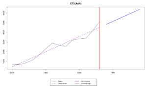
As we see, in this case the optimal smoothing parameters are equal to zero. This means that we do not take any information into account and just produce the straight line (deterministic trend). See for yourselves:

And here’s what happens with the admissible bounds:

es(M3$N0041$x,"AAN",bounds="a",h=6)

Time elapsed: 0.11 seconds
Model estimated: ETS(AAN)
Persistence vector g:
alpha  beta 
1.990 0.018 
Initial values were optimised.
5 parameters were estimated in the process
Residuals standard deviation: 327.758
Cost function type: MSE; Cost function value: 69059.107

Information criteria:
     AIC     AICc      BIC 
205.7283 213.2283 208.9236

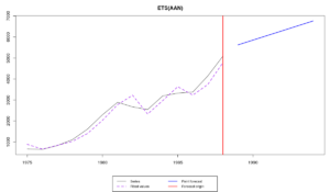
The smoothing parameter of the level, \(\alpha\) is greater than one. It is almost two. This means that the exponential smoothing is no longer averaging model, but I can assure you that the model is still stable. Such a high value of smoothing parameter means that the level in time series changes drastically. This is not common and usually not a desired, but possible behaviour of the exponential smoothing. Here how it looks:

Here I would like to note that model can be stable even with negative smoothing parameters. So don’t be scared. If the model is not stable, the function will warn you.

Last but not least, user can regulate values of B, lb and ub vectors for the first optimisation stage. Model selection does not work with the provided vectors of initial parameters, because the length of B, lb and ub vectors is fixed, while in the case of model selection it will vary from model to model. User also needs to make sure that the length of each of the vectors is correct and corresponds to the selected model. The values are passed via the ellipses, the following way:

B <- c(0.2, 0.1, M3$N0041$x[1], diff(M3$N0041$x)[1])
es(M3$N0041$x,"AAN",B=B,h=6,bounds="u")

Time elapsed: 0.1 seconds
Model estimated: ETS(AAN)
Persistence vector g:
alpha  beta 
    1     0 
Initial values were optimised.
5 parameters were estimated in the process
Residuals standard deviation: 429.923
Cost function type: MSE; Cost function value: 118821.938

Information criteria:
     AIC     AICc      BIC 
213.3256 220.8256 216.5209

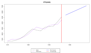
In this case we reached boundary values for both level and trend smoothing parameters. The resulting model has constantly changing level (random walk level) and deterministic trend. This is a weird, but possible combination. The fit and forecast looks similar to the model with the admissible bounds, but not as reactive:

Using this functionality, you may end up with ridiculous and meaningless models, so be aware and be careful. For example, the following does not have any sense from forecasting perspective:

B <- c(2.5, 1.1, M3$N0041$x[1], diff(M3$N0041$x)[1])
lb <- c(1,1, 0, -Inf)
ub <- c(3,3, Inf, Inf)
es(M3$N0041$x,"AAN",B=B, lb=lb, ub=ub, bounds="none",h=6)

Time elapsed: 0.12 seconds
Model estimated: ETS(AAN)
Persistence vector g:
alpha  beta 
2.483 1.093 
Initial values were optimised.
5 parameters were estimated in the process
Residuals standard deviation: 193.328
Cost function type: MSE; Cost function value: 24027.222

Information criteria:
     AIC     AICc      BIC 
190.9475 198.4475 194.1428 
Warning message:
Model ETS(AAN) is unstable! Use a different value of 'bounds' parameter to address this issue!

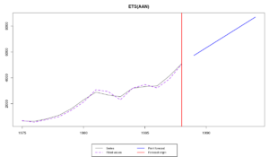
Although the fit is very good and the model approximates data better than all the others (MSE value is 24027 versus 70000 – 120000 of other models), the model is unstable (the function warns us about that), meaning that the weights are distributed in an unreasonable way: the older observations become more important than the newer ones. The forecast of such a model is meaningless and most probably is biased and not accurate. Here how it looks:

So be careful with manual tuning of the optimiser.

Have fun but be reasonable!