Three months have passed since the initial release of greybox on CRAN. I would not say that the package develops like crazy, but there have been some changes since May. Let’s have a look. We start by loading both greybox and smooth:

library(greybox)
library(smooth)

Rolling Origin

First of all, ro() function now has its own class and works with plot() function, so that you can have a visual representation of the results. Here’s an example:

x <- rnorm(100,100,10)
ourCall <- "es(data, h=h, intervals=TRUE)"
ourValue <- c("forecast", "lower", "upper")
ourRO <- ro(x,h=20,origins=5,ourCall,ourValue,co=TRUE)
plot(ourRO)

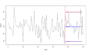
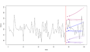
Each point on the produced graph corresponds to an origin and straight lines correspond to the forecasts. Given that we asked for point forecasts and for lower and upper bounds of prediction interval, we have three respective lines. By plotting the results of rolling origin experiment, we can see if the model is stable or not. Just compare the previous graph with the one produced from the call to Holt's model:

ourCall <- "es(data, model='AAN', h=h, intervals=TRUE)"
ourRO <- ro(x,h=20,origins=5,ourCall,ourValue,co=TRUE)
plot(ourRO)

Holt's model is not suitable for this time series, so it's forecasts are less stable than the forecasts of the automatically selected model in the previous case (which is ETS(A,N,N)).

Once again, there is a vignette with examples for the ro() function, have a look if you want to know more.

ALM - Advanced Linear Model

Yes, there is "Generalised Linear Model" in R, which implements Poisson, Gamma, Binomial and other regressions. Yes, there are smaller packages, implementing models with more exotic distributions. But I needed several regression models with: Laplace distribution, Folded normal distribution, Chi-squared distribution and one new mysterious distribution, which is currently called "S distribution". I needed them in one place and in one format: properly estimated using likelihoods, returning confidence intervals, information criteria and being able to produce forecasts. I also wanted them to work similar to lm(), so that the learning curve would not be too steep. So, here it is, the function alm(). It works quite similar to lm():

xreg <- cbind(rfnorm(100,1,10),rnorm(100,50,5))
xreg <- cbind(100+0.5*xreg[,1]-0.75*xreg[,2]+rlaplace(100,0,3),xreg,rnorm(100,300,10))
colnames(xreg) <- c("y","x1","x2","Noise")
inSample <- xreg[1:80,]
outSample <- xreg[-c(1:80),]

ourModel <- alm(y~x1+x2, inSample, distribution="laplace")
summary(ourModel)

Here's the output of the summary:

Distribution used in the estimation: Laplace
Coefficients:
            Estimate Std. Error Lower 2.5% Upper 97.5%
(Intercept) 95.85207    0.36746   95.12022    96.58392
x1           0.59618    0.02479    0.54681     0.64554
x2          -0.67865    0.00622   -0.69103    -0.66626
ICs:
     AIC     AICc      BIC     BICc 
474.2453 474.7786 483.7734 484.9419

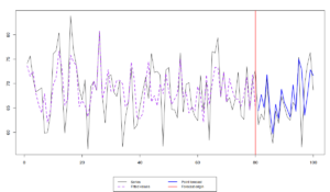
And here's the respective plot of the forecast:

plot(forecast(ourModel,outSample))

The thing that is currently missing in the function is prediction intervals, but this will be added in the upcoming releases.

Having the likelihood approach, allows comparing different models with different distributions using information criteria. Here's, for example, what model we get if we assume S-distribution (which has fatter tails than Laplace):

summary(alm(y~x1+x2, inSample, distribution="s"))

Distribution used in the estimation: S
Coefficients:
            Estimate Std. Error Lower 2.5% Upper 97.5%
(Intercept) 95.61244    0.23386   95.14666    96.07821
x1           0.56144    0.00721    0.54708     0.57581
x2          -0.66867    0.00302   -0.67470    -0.66265
ICs:
     AIC     AICc      BIC     BICc 
482.9358 483.4692 492.4639 493.6325

As you see, the information criteria for S distribution are higher than for Laplace, so we can conclude that the previous model was better than the second in terms of ICs.

Note that at this moment the AICc and BICc are not correct for non-normal models (at least the derivation of them needs to be double checked, which I haven't done yet), so don't rely on them too much.

I intent to add several other distributions that either are not available in R or are implemented unsatisfactory (from my point of view) - the function is written in a quite flexible way, so this should not be difficult to do. If you have any preferences, please add them on github, here.

I also want to implement the mixture distributions, so that things discussed in the paper on intermittent state-space model can also be implemented using pure regression.

Finally, now that I have alm, we can select between the regression models with different distributions (with stepwise() function) or even combine them using AIC weights (hello, lmCombine()!). Yes, I know that it sounds crazy (think of the pool of models in this case), but this should be fun!

Regression for Multiple Comparison with the Best

Please, note that this part of the post has been updated on 02.03.2020 in order to reflect the changes in the v0.5.9 version of the package.
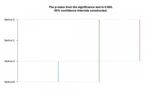
One of the typical tasks in forecasting is to evaluate the performance of different methods on the holdout. In order to do that, it is common to use some statistical tests, the most popular of which is Nemenyi / MCB (Multiple Comparison with the Best method). The test implemented in greybox package uses similar principles and relies on ranks of methods, but instead of taking averages and then applying studentised distances, it constructs a regression on the ranked data. This way we compare the median performance of different method (the same way as it is done in the classical MCB) and we produce parametric confidence intervals for parameters. The test is based on the simple linear model with dummy variables for each provided method (1 if the error corresponds to the method and 0 otherwise). Here's an example of how this thing works:

ourData <- cbind(rnorm(100,0,10), rnorm(100,-2,5), rnorm(100,2,6), rlaplace(100,1,5))
colnames(ourData) <- c("Method A","Method B","Method C","Method D")

ourTest <- rmcb(ourData, level=0.95)

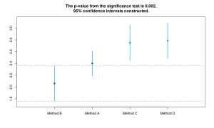
By default the function produces graph in the MCB (Multiple Comparison with the Best) style:

If we compare the results of the test with the mean rank values, we will see that they are the same:

apply(t(apply(ourData,1,rank)),2,mean)

Method A Method B Method C Method D 
    2.40     2.06     2.75     2.79

ourTest$mean

Method B Method A Method C Method D 
    2.06     2.40     2.75     2.79

This also reflects how the data was generated. Notice that Method D was generated from Laplace distribution with mean 1, but the test managed to give the correct answer in this situation, because Laplace distribution is symmetric and the sample size is large enough. But the main point of the test is that we can get the confidence intervals for each parameter, so we can see if the differences between the methods are significant: if the intervals intersect, then they are not.

The regression model used in the calculation is saved in the variable model and you can request a basic summary from it:

summary(ourTest$model)

            Estimate Std. Error  Lower 2.5% Upper 97.5%
(Intercept)     2.40  0.1083601  2.18761804  2.61238196
Method B       -0.34  0.1532444 -0.64035346 -0.03964654
Method C        0.35  0.1532444  0.04964654  0.65035346
Method D        0.39  0.1532444  0.08964654  0.69035346

But, please, keep in mind that this is not a proper "lm" object, so you cannot do much with it.

The function also reports p-value from the F-test of regression, testing the standard hypothesis that all the parameters are equal to zero.

We can also produce plots with vertical lines, that connect the models that are in the same group (no statistical difference, intersection of respective intervals). Here's the example for the same data:

plot(ourTest, outplot="lines")

If you want to tune the plot, you can always do this using the standart plot parameters:

plot(ourTest, xlab="Models", ylab="Errors")

Also, given that we work with a flexible plot method, you can tune the parameters of the canvas using "par()" function, as it is usually done in R.

What else?

Several methods have been moved from smooth to greybox. These include:

• pointLik() - returns point Likelihoods, discussed in our research with Nikos;
• pAIC, pBIC, pAICc, pBICc - point values of respective information criteria, from the same research;
• nParam() - returns number of the estimated parameters in the model (+ variance);
• errorType() - returns the type of error used in the model (Additive / Multiplicative);

Furthermore, as you might have already noticed, I've implemented several distribution functions:

• Folded normal distribution;
• Laplace distribution;
• S distribution.

Finally, there is also a function, called lmDynamic(), which uses pAIC in order to produce dynamic linear regression models. But this should be discussed separately in a separate post.

That's it for now. See you in greybox 0.4.0!