UPDATE: Starting from v2.5.1 the parameter intervals has been renamed into interval for the consistency purposes with the other R functions.

We have spent previous six posts discussing basics of es() function (underlying models and their implementation). Now it is time to move forward. Starting from this post we will discuss common parameters, shared by all the forecasting functions implemented in smooth. This means that the topics that we discuss are not only applicable to es(), but also to ssarima(), ces(), gum() and sma(). However, taking that we have only discussed ETS so far, we will use es() in our examples for now.

And I would like to start this series of general posts from the topic of prediction intervals.

Prediction intervals for smooth functions

One of the features of smooth functions is their ability to produce different types of prediction intervals. Parametric prediction intervals (triggered by interval="p", interval="parametric" or interval=TRUE) are derived analytically only for pure additive and pure multiplicative models and are based on the state-space model discussed in previous posts. In the current smooth version (v2.0.0) only es() function has multiplicative components, all the other functions are based on additive models. This makes es() “special”. While constructing intervals for pure models (either additive or multiplicative) is relatively easy to do, the mixed models cause pain in the arse (one of the reasons why I don’t like them). So in case of mixed ETS models, we have to use several tricks.

If the model has multiplicative error, non-multiplicative other components (trend, seasonality) and low variance of the error (smaller than 0.1), then the intervals can be approximated by similar models with additive error term. For example, the intervals for ETS(M,A,N) can be approximated with intervals of ETS(A,A,N), when the variance is low, because the distribution of errors in both models will be similar. In all the other cases we use simulations for prediction intervals construction (via sim.es() function). In this case the data is generated with preset parameters (including variance) and contains \(h\) observations. This process is repeated 10,000 times, resulting in 10,000 possible trajectories. After that the necessary quantiles of these trajectories for each step ahead are taken using quantile() function from stats package and returned as prediction intervals. This cannot be considered as a pure parametric approach, but it is the closest we have.

smooth functions also introduce semiparametric and nonparametric prediction intervals. Both of them are based on multiple steps ahead (also sometimes called as “trace”) forecast errors. These are obtained via producing forecasts for horizon 1 to \(h\) from each observation of time series. As a result a matrix with \(h\) columns and \(T-h\) rows is produced. In case of semi-parametric intervals (called using interval="sp" or interval="semiparametric"), variances of forecast errors for each horizon are calculated and then used in order to extract quantiles of either normal or log-normal distribution (depending on error type). This way we cover possible violation of assumptions of homoscedasticity and no autocorrelation in residuals, but we still assume that each separate observation has some parametric distribution.

In case of non-parametric prediction intervals (defined in R via interval="np" or interval="nonparametric"), we loosen assumptions further, dropping part about distribution of residuals. In this case quantile regressions are used as proposed by Taylor and Bunn, 1999. However we use a different form of regression model than the authors do:
\begin{equation} \label{eq:ssTaylorPIs}
\hat{e}_{j} = a_0 j ^ {a_{1}},
\end{equation}
where \(j = 1, .., h\) is forecast horizon. This function has an important advantage over the proposed by the authors second order polynomial: it does not have extremum (turning point) for \(j>0\), which means that the intervals won’t behave strangely after several observations ahead. Using polynomials for intervals sometimes leads to weird bounds (for example, expanding and then shrinking). On the other hand, power function allows producing wide variety of forecast trajectories, which correspond to differently increasing or decreasing bounds of prediction intervals (depending on values of \(a_0\) and \(a_1\)), without producing any ridiculous trajectories.

The main problem with nonparametric intervals produced by smooth is caused by quantile regressions, which do not behave well on small samples. In order to produce correct 0.95 quantile, we need to have at least 20 observations, and if we want 0.99 quantile, then the sample must contain at least 100. In the cases, when there is not enough observations, the produced intervals can be inaccurate and may not correspond to the nominal level values.

As a small note, if a user produces only one-step-ahead forecast, then semiparametric interval will correspond to parametric one (because only the variance of the one-step-ahead error is used), and the nonparametric interval is constructed using quantile() function from stats package.

Finally, the width of prediction intervals is regulated by parameter level, which can be written either as a fraction number (level=0.95) or as an integer number, less than 100 (level=95). I personally prefer former, but the latter is needed for the consistency with forecast package functions. By default all the smooth functions produce 95% prediction intervals.

There are some other features of prediction interval construction for specific intermittent models and cumulative forecasts, but they will be covered in upcoming posts.

Examples in R

We will use a time series N1241 as an example and we will estimate model ETS(A,Ad,N). Here’s how we do that:

ourModel1 <- es(M3$N1241$x, "AAdN", h=8, holdout=TRUE, interval="p")
ourModel2 <- es(M3$N1241$x, "AAdN", h=8, holdout=TRUE, interval="sp")
ourModel3 <- es(M3$N1241$x, "AAdN", h=8, holdout=TRUE, interval="np")

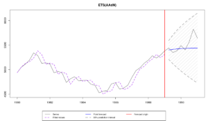
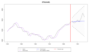
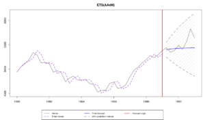
The resulting graphs demonstrate some differences in prediction intervals widths and shapes:

All of them cover actual values in the holdout, because the intervals are very wide. It is not obvious, which of them is the most appropriate for this task. So we can calculate the spread of intervals and see, which of them is on average wider:

mean(ourModel1$upper-ourModel1$lower)
mean(ourModel2$upper-ourModel2$lower)
mean(ourModel3$upper-ourModel3$lower)

Which results in:

950.4171
955.0831
850.614

In this specific example, the non-parametric interval appeared to be the narrowest, which is good, taking that it adequately covered values in the holdout sample. However, this doesn't mean that it is in general superior to the other methods. Selection of the appropriate intervals should be done based on the general understanding of the violated assumptions. If we didn't know the actual values in the holdout sample, then we could make a decision based on the analysis of the in-sample residuals in order to get a clue about the violation of any assumptions. This can be done, for example, this way:

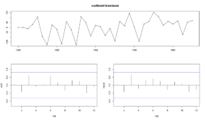
forecast::tsdisplay(ourModel1$residuals)

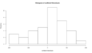
hist(ourModel1$residuals)

qqnorm(ourModel3$residuals)
qqline(ourModel3$residuals)

The first plot shows how residuals change over time and how the autocorrelation and partial autocorrelation functions look for this time series. There is no obvious autocorrelation and no obvious heteroscedasticity in the residuals. This means that we can assume that these conditions are not violated in the model, so there is no need to use semiparametric prediction intervals. However, the second and the third graphs demonstrate that the residuals are not normally distributed (as assumed by the model ETS(A,Ad,N)). This means that parametric prediction intervals may be wrong for this time series. All of this motivates the usage of nonparametric prediction intervals for the series N1241.

That's it for today.