Previously we’ve covered the basics of exogenous variables in smooth functions. Today we will go slightly crazy and discuss automatic variables selection. But before we do that, we need to look at a Santa’s little helper function implemented in smooth. It is called xregExpander(). It is useful in cases when you think that your exogenous variable may influence the variable of interest either via some lag or lead. Let’s say that we think that BJsales.lead discussed in the previous post influences sales in a non-standard way: for example, we believe that today’s value of sales is driven by the several values of that variable: the value today, five and 10 days ago. This means that we need to include BJsales.lead with lags. And xregExpander() from the greybox package allows automating this for us:

library("greybox")
newXreg <- xregExpander(BJsales.lead, lags=c(-5,-10))

The newXreg is a matrix, which contains the original data, the data with lag 5 and the data with lag 10. However, if we just move the original data several observations ahead or backwards, we will have missing values, so xregExpander() fills in those values with the forecasts using es() and iss() functions (depending on the type of variable we are dealing with). This also means that in cases of binary variables you may have weird averaged values as forecasts (e.g. 0.7812), so beware and look at the produced matrix. Maybe in your case it makes sense to just substitute these weird numbers with zeroes...

You may also need leads instead of lags. This is regulated with the same "lags" parameter but with positive values:

newXreg <- xregExpander(BJsales.lead, lags=c(7,-5,-10))

Once again, the values are shifted, and now the first 7 values are backcasted.

After expanding the exogenous variables, we can use them in smooth functions for forecasting purposes. All the rules discussed in the previous post apply:

es(BJsales, "XXN", xreg=newXreg, h=10, holdout=TRUE)

But what should we do if we have several variables and we are not sure what lags and leads to select? This may become a complicated task which can have several possible solutions. smooth functions provide one. I should warn you that this is not necessarily the best solution, but a solution. There is a function called stepwise() in greybox that does the selection based on an information criterion and partial correlations. In order to run this function the response variable needs to be in the first column. The idea of the function is simple, it works iteratively the following way:

1. The basic model of the first variable and the constant is constructed (this corresponds to simple mean). An information criterion is calculated;
2. The correlations of the residuals of the model with all the original exogenous variables are calculated;
3. The regression model of the response variable and all the variables in the previous model plus the new most correlated variable from (2) is constructed using lm() function;
4. An information criterion is calculated and is compared with the one from the previous model. If it is greater or equal to the previous one, then we stop and use the previous model. Otherwise we go to step 2.

This way we do not do a blind search, but we follow some sort of "trace" of a good model: if some significant part that can be explained by one of the exogenous variables is left in the residuals, then that variable is included in the model. Following correlations makes sure that we include only meaningful (from technical point of view) things in the model. Using information criteria allows overcoming the problem with the uncertainty of statistical tests. In general the function guarantees that you will have the model with the lowest information criterion. However this does not guarantee that you will end up with a meaningful model or with a model that produces the most accurate forecasts. And this is why evolution has granted human beings the almighty brain – it helps in selecting the most appropriate model in those cases, when statistics fails.

Let’s see how the function works with the same example and 1 to 10 leads and 1 to 10 lags (so we have 21 variables now). First we expand the data and form the matrix with all the variables:

newXreg <- as.data.frame(xregExpander(BJsales.lead,lags=c(-10:10)))
newXreg <- cbind(as.matrix(BJsales),newXreg)
colnames(newXreg)[1] <- "y"

This way we have a nice data frame with nice names, not something weird with strange long names. It is important to note that the response variable should be in the first column of the resulting matrix. After that we use our magical stepwise function:

ourModel <- stepwise(newXreg)

And here’s what it returns (the object of class “lm”):

Call:
lm(formula = y ~ xLag4 + xLag9 + xLag3 + xLag10 + xLag5 + xLag6 + 
    xLead9 + xLag7 + xLag8, data = newXreg)

Coefficients:
(Intercept)        xLag4        xLag9        xLag3       xLag10        xLag5        xLag6  
    17.6448       3.3712       1.3724       4.6781       1.5412       2.3213       1.7075  
     xLead9        xLag7        xLag8  
     0.3767       1.4025       1.3370

The values in the function are listed in the order of most correlated with the response variable to the least correlated ones. The function works very fast because it does not need to go through all the variables and their combinations in the dataset.

Okay. So, that’s the second nice function in smooth that you can use for exogenous variables. But what does it have to do with the main forecasting functions?

The thing is es(), ssarima(), ces(), ges() - all the forecasting functions in smooth have a parameter xregDo, which defines what to do with the provided exogenous variables, and by default it is set to "use". However, there is also an option of "select", which uses the aforementioned stepwise() function. The function is applied to the residuals of the specified model, and when the appropriate exogenous variables are found, the model with these variables is re-estimated. This may cause some inaccuracies in the selection mechanisms (because, for example, the optimisation of ETS and X parts does not happen simultaneously), but at least it is done in the finite time frame.

Let’s see how this works. First we use all the expanded variables for up to 10 lags and leads without the variables selection mechanism (I will remove the response variable from the first row of the data we previously used):

newXreg <- newXreg[,-1]
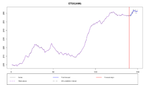
ourModelUse <- es(BJsales, "XXN", xreg=newXreg, h=10, holdout=TRUE, silent=FALSE, xregDo="use", intervals="sp")

Time elapsed: 1.13 seconds
Model estimated: ETSX(ANN)
Persistence vector g:
alpha 
0.922 
Initial values were optimised.
24 parameters were estimated in the process
Residuals standard deviation: 0.287
Xreg coefficients were estimated in a normal style
Cost function type: MSE; Cost function value: 0.068

Information criteria:
      AIC      AICc       BIC 
 69.23731  79.67209 139.83673 
95% semiparametric prediction intervals were constructed
100% of values are in the prediction interval
Forecast errors:
MPE: 0%; Bias: 55.7%; MAPE: 0.1%; SMAPE: 0.1%
MASE: 0.166; sMAE: 0.1%; RelMAE: 0.055; sMSE: 0%

As we see, the forecast became more accurate in this case than in the case of using pure BJsales.lead, which may mean that there can be a lagged relationship between the sales and the indicator. However, we have included too many exogenous variable, which may lead to the overfitting. So there is a potential for the accuracy increase if we remove the redundant variables. And that’s where the selection procedure kicks in:

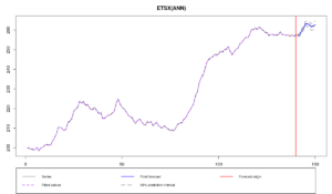
ourModelSelect <- es(BJsales, "XXN", xreg=newXreg, h=10, holdout=TRUE, silent=FALSE, xregDo="select", intervals="sp")

Time elapsed: 0.98 seconds
Model estimated: ETSX(ANN)
Persistence vector g:
alpha 
    1 
Initial values were optimised.
11 parameters were estimated in the process
Residuals standard deviation: 0.283
Xreg coefficients were estimated in a normal style
Cost function type: MSE; Cost function value: 0.074

Information criteria:
     AIC     AICc      BIC 
54.55463 56.61713 86.91270 
95% semiparametric prediction intervals were constructed
100% of values are in the prediction interval
Forecast errors:
MPE: 0%; Bias: 61.4%; MAPE: 0.1%; SMAPE: 0.1%
MASE: 0.159; sMAE: 0.1%; RelMAE: 0.052; sMSE: 0%

Although it is hard to see from graph, there is an increase in forecasting accuracy: MASE was reduced from 0.166 to 0.159. AICc has also reduced from 79.67209 to 56.61713. This is because only 8 exogenous variables are used in the second model (instead of 21):

ncol(ourModelUse$xreg)
ncol(ourModelSelect$xreg)

The xreg selection works even when you have combination of forecasts. The exogenous variables are selected for each model separately in this case, and then the forecasts are combined based on IC weights. For example, this way we can combine different non-seasonal additive ETS models:

ourModelCombine <- es(BJsales, c("ANN","AAN","AAdN","CCN"), xreg=newXreg, h=10, holdout=TRUE, silent=FALSE, xregDo="s", intervals="sp")

Time elapsed: 1.46 seconds
Model estimated: ETSX(CCN)
Initial values were optimised.
Residuals standard deviation: 0.272
Xreg coefficients were estimated in a normal style
Cost function type: MSE

Information criteria:
(combined values)
     AIC     AICc      BIC 
54.55463 56.61713 86.91270 
95% semiparametric prediction intervals were constructed
100% of values are in the prediction interval
Forecast errors:
MPE: 0%; Bias: 61.4%; MAPE: 0.1%; SMAPE: 0.1%
MASE: 0.159; sMAE: 0.1%; RelMAE: 0.052; sMSE: 0%

Taking that ETSX(A,N,N) is significantly better in terms of AICc than the other models, we end up with a maximum weight for that model and infinitesimal weights for the others. That’s why the forecasts of the ourModelSelect and ourModelCombine are roughly the same. Starting from v2.3.2, es() function returns the matrix of information criteria for different models estimated in the process, so we can see what was used and what were the values for the models. This information is available through the element ICs:

ourModelCombine$ICs

               AIC      AICc      BIC
ANN       54.55463  56.61713  86.9127
AAN      120.85273 122.91523 153.2108
AAdN     107.76905 110.22575 143.0688
Combined  54.55463  56.61713  86.9127

So, as we see, ETS(A,N,N) had indeed the lowest information criterion of all the models in the combination (substantially lower than the others), which led to its domination in the combination.

Keep in mind that this combination of forecasts does not mean the combination of regression models with different exogenous variables – this functionality is currently unavailable, and I am not sure how to implement it (and whether it is needed at all). The combination of forecasts is done for the whole ETS models, not just for the X parts of it.

Finally, it is worth noting that the variables selection approach we use here puts more importance on the dynamic model (in our examples it is ETS) rather than on the exogenous variables. We use exogenous variables as an additional instrument which allows increasing the forecasting accuracy. The conventional econometrics approach would be the other way around: construct regression, then add dynamic components to that in case you cannot explain the response variable with the available data. This approach has different aims and leads to different results.