Authors: Ivan Svetunkov, Nikolaos Kourentzes, Keith Ord.

Journal: Naval Research Logistics

Abstract: Exponential smoothing has been one of the most popular forecasting methods used to support various decisions in organisations, in activities such as inventory management, scheduling, revenue management and other areas. Although its relative simplicity and transparency have made it very attractive for research and practice, identifying the underlying trend remains challenging with significant impact on the resulting accuracy. This has resulted in the development of various modifications of trend models, introducing a model selection problem. With the aim of addressing this problem, we propose the Complex Exponential Smoothing (CES), based on the theory of functions of complex variables. The basic CES approach involves only two parameters and does not require a model selection procedure. Despite these simplifications, CES proves to be competitive with, or even superior to existing methods. We show that CES has several advantages over conventional exponential smoothing models: it can model and forecast both stationary and non-stationary processes, and CES can capture both level and trend cases, as defined in the conventional exponential smoothing classification. CES is evaluated on several forecasting competition datasets, demonstrating better performance than established benchmarks. We conclude that CES has desirable features for time series modelling and opens new promising avenues for research.

Working paper

DOI: 10.1002/nav.22074

The story of the paper.

The idea of Complex Exponential Smoothing

One of the most fundamental ideas in forecasting is the decomposition of time series into several unobservable components (see, for example, Section 3.1 of ADAM monograph), typically: level, trend, seasonality, error. ETS relies on this idea of decomposition and implements the selection of components via information criteria. However, not all time series have these components and the split itself is arbitrary, because, for example, in practice time series with slow trend might be indistinguishable from the series with rapidly changing level. Furthermore, in reality, the data can be more complicated – it might not have distinct level and trend, and instead can represent a non-linear mixture of unobservable components.

Complex Exponential Smoothing models non-linearity in time series and captures a structure in a different way. Here is how the conventional CES method is formulated:

\begin{equation} \label{eq:cesalgebraic}
\hat{y}_{t} + i \hat{e}_{t} = (\alpha_0 + i\alpha_1)(y_{t-1} + i e_{t-1}) + (1 – \alpha_0 + i – i\alpha_1)(\hat{y}_{t-1} + i \hat{e}_{t-1}) ,
\end{equation}
where \(y_t\) is the actual value, \(e_t\) is the forecast error, \(\hat{y}_t\) is the predicted value, \(\hat{e}_t\) is proxy for the error term, \(\alpha_0\) and \(\alpha_1\) are the smoothing parameters and \(i\) is the imaginary unit, satisfying the equation \(i^2=-1\). Due to the usage of complex variables, the method allows distributing weights between the observations over time in a non-linear way. This becomes more apparent if we insert the same formula \eqref{eq:cesalgebraic} in the right hand side of \eqref{eq:cesalgebraic} and do that several times to get a recursion (similar how it is typically done for Simple Exponential Smoothing. See for, example, Subsection 3.4.2 of ADAM monograph):
\begin{equation} \label{eq:cesalgebraicExpanded}
\begin{aligned}
\hat{y}_{t} + i \hat{e}_{t} = & (\alpha_0 + i\alpha_1)(y_{t-1} + i e_{t-1}) + \\
& (\alpha_0 + i\alpha_1) (1 – \alpha_0 + i – i\alpha_1) (y_{t-2} + i e_{t-2}) + \\
& (\alpha_0 + i\alpha_1) (1 – \alpha_0 + i – i\alpha_1)^2 (y_{t-3} + i e_{t-3}) + \\
& … + \\
& (\alpha_0 + i\alpha_1) (1 – \alpha_0 + i – i\alpha_1)^{t-2} (y_{1} + i e_{1}) + \\
& (1 – \alpha_0 + i – i\alpha_1)^{t-1} (\hat{y}_{1} + i \hat{e}_{1}) .
\end{aligned}
\end{equation}
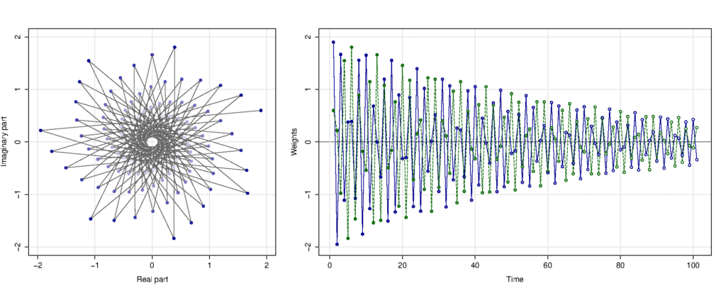
This exponentiation of \((1 – \alpha_0 + i – i\alpha_1)\) in the formula above is what distributes the weights over time in a non-linear fashion. All of this is difficult to understand, so here is a beautiful figure showing how the weights can be distributed over time (blue line – weights for the actual value, green one – weights for the forecast errors):

Depending on values of the complex smoothing parameter \(\alpha_0 + i\alpha_1\), the distribution of weights will have different shape. It does not need to be harmonic as on the plot above, it can also be classical exponential (as in Simple Exponential Smoothing), which is achieved, when \(\alpha_1\) is close to one. This is what gives CES its flexibility and allows it deal with both stationary and non-stationary time series, without a need of switching between time series components.

The published paper also discusses a seasonal modification of CES model, which introduces seasonal component that can act either as additive, or multiplicative, or something in-between the two. I do not provide the formula here, because it is cumbersome.

Examples in R

In R, CES is implemented in ces() of smooth package. There is also auto.ces() function which does selection between seasonal and non-seasonal models using information criteria. The syntax of the function is similar to the one of es() and adam(). Here is an example of its application:

cesModel <- smooth::auto.ces(BJsales, holdout=TRUE, h=12)
cesModel

Time elapsed: 0.05 seconds
Model estimated: CES(n)
a0 + ia1: 1.9981+1.0034i
Initial values were produced using backcasting.

Loss function type: likelihood; Loss function value: 249.4613
Error standard deviation: 1.4914
Sample size: 138
Number of estimated parameters: 3
Number of degrees of freedom: 135
Information criteria:
     AIC     AICc      BIC     BICc 
504.9227 505.1018 513.7045 514.1457 

Forecast errors:
MPE: 0%; sCE: 0.7%; Asymmetry: -5%; MAPE: 0.4%
MASE: 0.857; sMAE: 0.4%; sMSE: 0%; rMAE: 0.329; rRMSE: 0.338

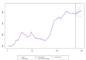
The output above has been discussed on this website in the context of es() in this post. The main difference is in the reported parameter. We see that \(\alpha_0 + i\alpha_1 = 1.9981 + i 1.0034\). The estimated model can then be used in forecasting, for example, using the command:

cesModel |> forecast(h=12, interval="p") |> plot()

to get:

This function hasn't changed since I finished my PhD in 2016, so the results in terms of its accuracy discussed in this post still hold. It does not perform stellar, but as Petropoulos & Svetunkov (2020) showed, it brings value in combination of models. This is because CES captures well the long term tendencies in time series.

Last but not least, I plan to update the code of ces() as a part of the move to more efficient C++ routine in the smooth package in v3.2.0. So, its performance will change slightly but probably will not change much.

Acknowledgments

As a final word, I am immensely grateful to Nikolaos Kourentzes, who believed in CES back in 2012 and supported me throughout these years, during my PhD and after it without hesitation. I am also grateful to Keith Ord who helped in improving the paper and making it happen in the end. Finally, I am grateful to my father, Sergey Svetunkov, who provided me guidance in my first steps in academia and believed in my research, when it wasn't even fashionable.

If you want to know more about CES, read the paper (you can do it here as well) or read the story of the paper.