


Sometimes, when you need to forecast demand, you may notice that the recorded data contains zeroes. There are several possible reasons for this, but today we’ll briefly discuss one of them. Welcome to the world of “intermittent demand”!
Intermittent demand is the demand that happens at irregular frequency (Svetunkov & Boylan, 2023). This means you cannot predict when demand occurs: you might have some sales of a lipstick on Monday but then nothing on Tuesday, and there is no pattern in purchases. This additional element of randomness, not only about how much but also when people buy, creates additional challenges. Intermittent demand can be split into two parts: demand sizes (how much is needed) and demand occurrence (when it is needed) or demand intervals (the time between purchases).
If your demand has zeroes for some specific reasons, such as certain times of day, it may be non-intermittent. Zeroes can also result from shortages or recording errors, which should be treated differently. In those cases, the demand itself maybe non-zero, but sales would be zero due to technical reasons. This means that not every series that has zeroes should be considered and treated as intermittent.
An important thing to note is that intermittent demand is not the same as count demand, but it is a wider term. Zero value in case of count data is just a possible outcome, e.g. nobody came to the hospital at this hour because there was no demand, and thus we recorded a zero value. In fact, it is possible for count demand not to have any zeroes at all, while for the intermittent it is a requirement. Furthermore, zero has a slightly different meaning in the intermittent demand: there might be a potential non-zero demand for paracetamol at our shop at this hour, but we just did not observe it because a customer didn’t make it to the shop. The difference between the two situations is intricate, but fundamental. However it is worth noting that intermittent demand can be either count or non-count. For example, demand for jet engines is count, while demand for EV charging is non-count.
The fundamental difference between count demand and intermittent demand lies in their treatment. In intermittent demand, you may need separate models for demand occurrence and demand sizes. In count demand, using an appropriate count distribution model (e.g., Poisson or Negative Binomial) or an ML method is sufficient. The split into demand sizes and demand occurrence (or demand intervals) gives additional flexibility and allows capturing more complex patterns in the data. For example, the frequency of purchase might increase if the product becomes more popular, implying that the probability of sale goes up, but the demand sizes might stay on a similar level. Another situation would be when product becomes obsolete, where both demand sizes and demand occurrence decline over time. Finally, there is also a possibility of demand having the same level of occurrence, not changing substantially over time (e.g. sales of large machines). All of these cases can be captured using models that split demand into two aforementioned parts.
The following image provides several examples of intermittent demand, which we will discuss in future posts:
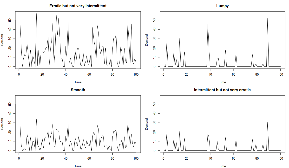
Examples of intermittent demand data
Finally, intermittent demand can appear at higher recording frequencies. For instance, while daily demand may seem regular, hourly data may reveal zeroes. This increases forecasting complexity, so when selecting an aggregation level, we should consider whether the added complexity aligns with the decision-making based on the forecasts.
Additional resources to read: a post about measuring accuracy of intermittent demand, a monograph on intermittent demand forecasting by Boylan & Syntetos.