Theoretical stuff

Last time we talked about pure additive models, today I want to discuss multiplicative ones.

There is a general scepticism about pure multiplicative exponential smoothing models in the forecasters society, because it is not clear why level, trend, seasonality and error term should be multiplied. Well, when it comes to seasonality, then there is no doubt – multiplicative one is more often met than additive and thus is more often used in practice. However, multiplicative trend and multiplicative error are not as straight forward, because it is not easy to understand why we need them in the first place. In addition, models with these multiplicative components are harder to implement, harder to work with and their forecast accuracy is not necessarily better than accuracy of other models.

So why bother at all? There is at least one reason. Pure multiplicative models are constructed with the assumption that the data we work with is positive only. And this is a plausible assumption when we work with demand on products, because selling -50 boots in March 2017 or something like that does not make much sense. However, when we work with high scale data (for example, hundreds or even thousands of units), then this advantage becomes negligible, so pure additive or mixed models can be used instead. This, in fact, is the reason why pure multiplicative models are neglected.

So, what’s the catch with these models? Let’s have a look.

The general pure multiplicative model can be written in the following compact form, if we use natural logarithms:
\begin{equation} \label{eq:ssGeneralMultiplicative}
\begin{matrix}
y_t = \exp \left(w’ \log(v_{t-l}) + \log(1+\epsilon_t) \right) \\
\log(v_t) = F \log(v_{t-l}) + \log (1 + g \epsilon_t)
\end{matrix} ,
\end{equation}
where all the notations have already been introduced in the previous post. The only thing to note is that both \(\exp\) and \(\log\) are applied element wise to vectors. This means that \(\log(v_t)\) will result in vector consisting of components in logarithms. The important thing to note here is that all the components of this models must be positive, otherwise it won’t work.

An example of multiplicative model written in this form is ETS(M,M,N) – model with multiplicative error and multiplicative trend – can be written as:
\begin{equation} \label{eq:ssETS(M,M,N)}
\begin{matrix}
y_t = \exp \left(\log(l_{t-l}) + \log(b_{t-l}) + \log(1 + \epsilon_t) \right) \\
\log(l_t) = \log(l_{t-l}) + \log(b_{t-l}) + \log (1 + \alpha \epsilon_t) \\
\log(b_t) = \log(b_{t-l}) + \log (1 + \beta \epsilon_t)
\end{matrix} .
\end{equation}
Taking exponent of second and third equations and simplifying the first one in \eqref{eq:ssETS(M,M,N)} leads to the conventional model, that underlies Pegel’s method:
\begin{equation} \label{eq:ssETS(M,M,N)_Pegels}
\begin{matrix}
y_t = l_{t-l} b_{t-l} (1 + \epsilon_t) \\
l_t = l_{t-l} b_{t-l} (1 + \alpha \epsilon_t) \\
b_t = b_{t-l} (1 + \beta \epsilon_t)
\end{matrix} .
\end{equation}
Multiplication of level, trend and error term restricts actuals with positive values, but this will only be true if we impose correct assumptions on error term. While Hyndman et al. 2008 assume that it is distributed normally (they have actually discussed other assumption in Chapter 15), we assume in es() that it is distributed log-normally:
\begin{equation} \label{eq:ssErrorlogN}
(1 + \epsilon_t) \sim \text{log}\mathcal{N}(0,\sigma^2),
\end{equation}
where \(\sigma^2\) is variance of logarithm of \(1 + \epsilon_t\). Why log-normal distribution? Let me explain. When the variance \(\sigma^2\) is small, the differences between es() and ets() models with multiplicative error are almost non-existent, because in this case both normal and log-normal distributions look very similar. However with larger variance the differences become more substantial (and by larger I mean something greater than 0.1), because log-normal distribution becomes positive skewed with a longer tail. In addition, with a higher variance and normality assumption chances of having \(1 + \epsilon_t \leq 0\) increase, which contradicts the original model. So the assumption of normality is not always unrealistic and may lead to problems in model construction. That is why we need the assumption \eqref{eq:ssErrorlogN}.

Now \eqref{eq:ssErrorlogN} influences several aspects of how the model work: point forecasts, prediction intervals and estimation of the model \eqref{eq:ssGeneralMultiplicative} will be slightly different.

First of all, with low actual values point forecasts correspond to median rather than mean. This is because of relations between mean in normal and log-normal distributions and the fact that variance of error term in these cases may become sufficiently large for them to differ substantially. Arguably, median is what we need in cases of skewed distributions and that’s what es() produces. Knowing that is especially important in cases with intermittent demand models, which will be discussed in this blog at some distant point in future.

Secondly, due to asymmetry of log-normal distribution prediction intervals become asymmetric. This will especially be evident, when scale of data is low and variance is high. In the other situations the intervals will be very close to intervals produced by additive error models with normally distributed errors.

Finally, the estimation of models with multiplicative errors should be based on the following concentrated log-likelihood function (for log-normal distribution):
\begin{equation} \label{eq:ssConcentratedLogLikelihoodLnorm}
\ell(\theta | Y) = -\frac{T}{2} \left( \log \left( 2 \pi e \right) +\log \left( \hat{\sigma}^2 \right) \right) -\sum_{t=1}^T \log y_t ,
\end{equation}
where \(\hat{\sigma}^2 = \frac{1}{T} \sum_{t=1}^T \log^2(1 + \epsilon_{t})\). The likelihood function \eqref{eq:ssConcentratedLogLikelihoodLnorm} looks very similar to the one used in additive models, but leads to a slightly different cost function (that we need to minimise):
\begin{equation} \label{eq:ssCostFunction}
\text{CF} = \log \left( \hat{\sigma}^2 \right) + \frac{2}{T} \sum_{t=1}^T \log y_t .
\end{equation}
Giving interpretation to the cost function \eqref{eq:ssCostFunction}, variance of error term here is weighed with actual values. So roughly saying higher actuals will be predicted with higher precision.

R stuff

A good example of data, where pure multiplicative model can be used is time series N2457 from M3. Although the scale of data is high (the average is around 5000), the variability of data is high as well, which indicates that multiplicative model could be efficiently used here. So, let’s construct the ETS(M,N,N) model with parametric prediction intervals:

es(M3$N2457$x, "MNN", h=18, holdout=TRUE, intervals="p")

This results in the following output:

Time elapsed: 0.1 seconds
Model estimated: ETS(MNN)
Persistence vector g:
alpha 
0.145 
Initial values were optimised.
3 parameters were estimated in the process
Residuals standard deviation: 0.413
Cost function type: MSE; Cost function value: 1288657

Information criteria:
     AIC     AICc      BIC 
1645.978 1646.236 1653.702 
95% parametric prediction intervals were constructed
72% of values are in the prediction interval
Forecast errors:
MPE: 26.3%; Bias: 87%; MAPE: 39.8%; SMAPE: 49.4%
MASE: 2.944; sMAE: 120.1%; RelMAE: 1.258; sMSE: 242.7%

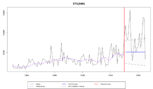
We have already discussed what each of the lines of this output means in the previous post, so we will not stop on that here. The thing to note, however, is the line with residuals standard deviation, which is equal to 0.413 (meaning that variance is approximately equal to 0.17). With this standard deviation the distribution will be noticeably skewed. This can be evidently seen on the produced graph:

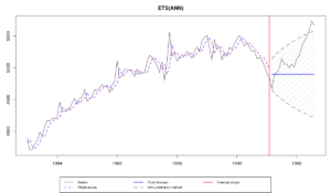
For the same time series ETS(A,N,N) model will produce the following forecast:

Comparing the two graphs, we can notice that prediction intervals on the first one are more adequate for this data, because they take into account skewness in errors distribution. As a result they cover more observations in the holdout than the intervals of the second model.

A counter example is time series N2348 – it does not have as high variability as N2457, so ETS(M,N,N) and ETS(A,N,N) produce very similar point forecasts and prediction intervals. This is because variance in multiplicative model applied to this data is equal to 0.000625 and as a result the log-normal distribution becomes very close to the normal. See for yourselves:

So in cases of time series similar to N2348 both multiplicative and additive error models can be used equally efficiently. But in general pure multiplicative models should not be neglected as they have useful properties. In one of the next posts we will see that these properties become especially useful for intermittent demand.

That’s all, folks!