Mixed models

In the previous posts we have discussed pure additive and pure multiplicative exponential smoothing models. The next logical step would be to discuss mixed models, where some components have additive and the others have multiplicative nature. But we won’t spend much time on them because I personally think that they do not make much sense. Why do I think so? Well, they simply contradict basic modelling logic. For example, the original Holt-Winters method, which has underlying ETS(A,A,M) model, assumes that data may be both positive and negative (from side of additive error and trend), but at the same time does not work when data is non-positive (because multiplicative seasonality cannot be calculated in this case). This causes severe problems in forecasting of data with low values. A simple example is dying out seasonal product, which implies negative trend, low values and some periodic pattern. In this case level and trend components may become negative, which screws the seasonality. Having said that, mixed models work fine when data has high level. But this disadvantage of mixed models should be taken into account when one of them is selected. And this is a reason why I don’t want to spend a separate post on them. This paragraph should suffice.

Theory of model selection and combinations

Now that we have discussed all the possible types of exponential smoothing models, it is time to select the most appropriate one for your data. Fotios Petropoulos and Nikos Kourentzes had a research on this topic and demonstrated that human beings are very good in selecting appropriate components for each time series. However when a forecaster faces thousands of products that he needs to work with, it is not possible to select components individually. That’s why automatic model selection is needed.

There are many model selection methods and a lot of literature on this topic. I have implemented only one of those methods in es() function. It is based on information criteria calculation and proved to work well (Hyndman et al. 2002, Billah et al. 2006). Any information criterion uses likelihood function, that is why I showed them in the previous posts. These likelihoods depend mainly on error term, so mixed models will have one of two likelihood functions.

es() allows selecting between AIC (Akaike Information Criterion), AICc (Akaike Information Criterion corrected) and BIC (Bayesian Information Criterion, also known as Schwarz IC). The very basic information criterion is AIC. It is calculated for a chosen model using formula:
\begin{equation} \label{eq:AIC}
\text{AIC} = -2 \ell \left(\theta, \hat{\sigma}^2 | Y \right) + 2k,
\end{equation}
where \(k\) is number of parameters of the model. Not going too much into details, the model with the smallest AIC is considered to be the closest to the true model. Obviously IC cannot be calculated without model fitting, which implies that a human being needs to form a pool of models, then fit each of them to the data, calculate an information criterion for each of them and after that select the one model that has the lowest IC value. There are 30 ETS models, so this procedure may take some time. Or even too much time, if we deal with large samples. So what can be done in order to increase the speed?

I have decided to solve this problem using logic and decrease pool of models in several steps. Here’s what happens in es():

1. Simple ETS(A,N,N) is fitted to the data.
2. ETS(A,N,A) is fitted to the data.

If IC of (2) is lower than IC of (1), then there is some type of seasonality in the data. This means that we can exclude non-seasonal models. This decreases pool of models from 30 to 20. After that we go to step (3).

Otherwise there is no seasonality in the data, which means that the pool of models decreases from 30 to 10. We go to step (4).

These two steps need some explanation. We do not discuss trend at this point because even if data is trended, then ETS(A,N,N) will be a fine approximator for it (but a very poor forecaster, which is irrelevant at this point). The smoothing parameter in this case will obviously be very high (can be very close to 1), but this is not really important when we want to see if there is seasonality in the data. ETS(A,N,A) will perform better than ETS(A,N,N) on series with trend and seasonality. Similar argument holds even when data has multiplicative seasonality. ETS(A,N,A) in this case will have lower IC than ETS(A,N,N), because it will always fit seasonal data better.

3. Fit ETS(A,N,M). Compare it with (2).

If IC of (3) is lower than (2), then seasonality has multiplicative type. This reduces pool of models from 20 to 10. Go to step (4).

Otherwise, multiplicative seasonality does not contribute in the model, we can stick with additive, decreasing pool of models to 10. Go to step (4).

The logic here is similar to the previous step. If there is trend with multiplicative seasonality in the data, then level part of the model will capture the increase of level, while the model with multiplicative seasonality will approximate data better than the one with additive.

4. Fit a model with additive trend and preselected type of seasonality. Depending on steps (2) and (3) this can either be ETS(A,A,N), ETS(A,A,A) or ETS(A,A,M).

If IC of this step model is lower than IC of model selected on previous step, then there is a trend in data. This decreases pool of models from 10 to 8.

Otherwise there is no trend, meaning that we deal either with model with additive or multiplicative error. The pool of models decreases from 10 to 1. For example, if we compared ETS(A,A,M) and (A,N,M), and found that the latter is better, then ther is only one model left to fit and compare with others – ETS(M,N,M).

Additive trend on the last step is a good approximation for all trend types. If we find that it contributes towards better fit, then we can investigate, what type of trend is needed. Also, because we have already identified seasonality type, it won’t make any distortions on this step.

Using this algorithm of model selection allows to fit from 5 to 12 models instead of 30. The experiments that I have conducted showed that this way we usually end up with a model with the lowest IC. Keep in mind that this does not necessarily mean that the chosen model will produce the most accurate forecasts. Here we only care for the fit and closeness to the “true model”. Which brings us to another idea. We know from forecasting theory that combinations of forecasts are on average more accurate than individual models. So why not use them for ETS?

One of the simplest and pretty efficient methods would be to produce forecasts from each model in the pool, then combine them and return the final combined forecast. The combination itself can be done with either equal weights or unequal ones. The former does not make much sense, when we deal with data with specific components (for example, why would ETS(A,N,N) have the same weight as ETS(A,N,A) on seasonal data?). So we need to use some weights. There is a lot of methods of weights distribution, but we will use the one discussed in Burnham and Anderson (2002), which is based on information criteria, so we do not create anything artificial and just use what ETS models implemented in es() already have. Weights for each produced forecast are calculated using the following formula:
\begin{equation} \label{eq:statLikelihoodAICweights}
w_j = \frac{ \exp \left(-\frac{1}{2} \left(\text{IC}_j -\min(\text{IC}) \right) \right)}{\sum_{i=1}^m \exp \left(-\frac{1}{2} \left(\text{IC}_i -\min(\text{IC}) \right) \right)},
\end{equation}
where \(m\) is number of models in the pool, IC\(_j\) is information criterion value for \(j^{th}\) model and \(\min(\text{IC})\) is the value of the lowest IC in the pool. Models with lower IC will have higher weights than the ones with high ICs. These weights are then used for combination of forecasts, prediction intervals and fitted values. Any information criterion among discussed above can be used instead of IC.

By the way, Stephan Kolassa (2011) showed that using this method of forecasts combination increases accuracy of ETS models. This method protects forecaster from a random error, where a wrong model would be chosen for some unknown reasons. The pool of models is determined by a forecaster and may either include all the 30 ETS models or a sub-sample of them.

Practice of model selection and combinations

Now that we have discussed basics of model selection and combinations, we can try it out in es() function. There are several ways of making this selection. Let’s start from the very basic one.

If we are not sure what to do and whether we need to restrict our models, we may use default selection mechanism, which is triggered by setting all the components of the model parameter equal to “Z”. This is taken from Rob Hyndman ets() function which uses the same notation. If we ask for model=”ZZZ”, then es() function will use the described in the previous section model selection algorithm.

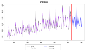
For example, for a time series N2568 from M3 we will have:

es(M3$N2568$x, "ZZZ", h=18)

Which results in:

Forming the pool of models based on... ANN, ANA, ANM, AAM, Estimation progress: 100%... Done! 
Time elapsed: 2.6 seconds
Model estimated: ETS(MMdM)
Persistence vector g:
alpha  beta gamma 
0.020 0.020 0.001 
Damping parameter: 0.965
Initial values were optimised.
19 parameters were estimated in the process
Residuals standard deviation: 0.065
Cost function type: MSE; Cost function value: 169626

Information criteria:
     AIC     AICc      BIC 
1763.990 1771.907 1816.309 

During the model selection the function will print out the progress and tell us what’s happening: first it tries “ANN”, then “ANA”, then “ANM” (which means that the data is seasonal and it tries to define type of seasonality) and finally “AAM” (checking the trend). If we do not need any output we can ask our function to shut up by specifying parameter silent=”all”. As we see, the optimal model for this data is ETS(M,Md,M).

Note that the mentioned model selection algorithm is only used when we specify “Z” for at least one component and either “Z” or “A”, or “M”, or “N” for the others. Setting some components equal to either “A”, “M” or “N” will speed up the selection process, but the function will use the discussed above selection algorithm.

By default the selection is done using AICc, but AIC and BIC are also available and can be selected with ic parameter:

es(M3$N2568$x, "ZZM", h=18, ic="BIC")

Now let’s assume that for some reason we are only interested in pure additive models. What should we do in this case? How can we select the best model from such a pool of 6 models? es() function allows us to do that via “X” component:

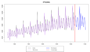
es(M3$N2568$x, "XXX", h=18)

This gives us:

Estimation progress: 100%... Done! 
Time elapsed: 0.72 seconds
Model estimated: ETS(ANA)
Persistence vector g:
alpha gamma 
0.174 0.695 
Initial values were optimised.
16 parameters were estimated in the process
Residuals standard deviation: 609.711
Cost function type: MSE; Cost function value: 320472

Information criteria:
     AIC     AICc      BIC 
1831.789 1837.284 1875.847

In this case the model selection algorithm described in the previous section is not used. We just check 6 models and select the best of them. The pool of models in this case includes: “ANN”, “AAN”, “AAdN”, “ANA”, “AAA” and “AAdA”. For this data the best model in this pool is ETS(A,N,A).

In a similar manner we can ask the function to select between multiplicative models only. This is regulated with “Y” value for components:

es(M3$N2568$x, "YYY", h=18)

Similar to “XXX” we go through 6 models and select the best one. In this case we will end up with exactly the same model as in “ZZZ” case, because the optimal model for this time series is ETS(M,Md,M). “YYY” can be especially useful, when we deal with low level values.

Now that we know these features, we can combine different parameters and form pools that we want. For example, we can select the best model between “MNN”, “MAN”, “MAdN”, “MNM”, “MAM”, MAdM this way:

es(M3$N2568$x, "YXY", h=18)

Which results in:

Estimation progress: 100%... Done! 
Time elapsed: 0.92 seconds
Model estimated: ETS(MAdM)
Persistence vector g:
alpha  beta gamma 
0.021 0.021 0.001 
Damping parameter: 0.976
Initial values were optimised.
19 parameters were estimated in the process
Residuals standard deviation: 0.065
Cost function type: MSE; Cost function value: 169730

Information criteria:
     AIC     AICc      BIC 
1764.062 1771.979 1816.380 

Note that the information criteria for ETS(M,Ad,M) are very close to the optimal ETS(M,Md,M). This raises the question which of the models to prefer if the difference between them is negligible…

We can also pre-specify some components if we really want something special. For example, anything with multiplicative seasonality:

es(M3$N2568$x, "ZZM", h=18)

Finally, there is another way to select the best model from some pre-specified pool. Let’s say that we have a favourite set of ETS models that we want to check, which includes: “ANN”, “MNN”, “AAdN”, “AAdM” and “MMdM”. This cannot be specified via “X”, “Y” and “Z” parameters, but it can be provided to es() as a vector of model names:

es(M3$N2568$x, c("ANN", "MNN", "AAdN", "AAdM", "MMdM"), h=18)

In this case the function will go through all the provided models and select the one with the lowest IC (which is ETS(M,Md,M) in this case).

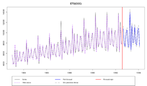
Now let’s have a look at combinations. This is specified with components equal to “C”. Once again we can set a pool of models via “Z”, “X”, “Y”, “N”, “A” and “M” and combine their forecasts. In order to produce combinations we need to specify at least one component as “C”. In a very simple case we have (let’s also ask for prediction intervals in order to see how this thing works):

es(M3$N2568$x, "CCC", h=18, intervals=TRUE)

With the following output:

Estimation progress: 100%... Done!
Time elapsed: 10.04 seconds
Model estimated: ETS(CCC)
Initial values were optimised.
Residuals standard deviation: 438.242
Cost function type: MSE

Information criteria:
Combined AICc 
     1772.198 
95% parametric prediction intervals were constructed

and graph:

Because we have set “C” for all the components, we have combined point forecasts and prediction intervals for all the 30 models, which took almost 10 seconds. But we could have asked something stricter, if we knew that some of the components need to be of a specific type. For example, additive seasonality does not make much sense for our time series, so we can ask for:

es(M3$N2568$x, "CCM", h=18)

which will use only 10 models and as a result happen approximately 3 times faster with approximately the same result for our time series, which exhibits obvious multiplicative seasonality. This means that all the models with multiplicative seasonality will have higher weight than other models.

We can also use “X” and “Y”, which in this case will ask our function to use additive and multiplicative models in combinations respectively. For example, this thing:

es(M3$N2568$x, "CXY", h=18)

will combine forecasts from the following 12 models: “ANN”, “AAN”, “AAdN”, “ANM”, “AAM”, “AAdM”, “MNN”, “MAN”, “MAdN”, “MNM”, “MAM”, “MAdM”.

Finally forecasts can be combined from an arbitrary pool of models. In order to do that a user needs to add “CCC” model in the desired pool of models. Here how it works:

es(M3$N2568$x, c("CCC","ANN", "MNN", "AAdN", "AAdM", "MMdM"), h=18)

This will combine forecasts of “ANN”, “MNN”, “AAdN”, “AAdM” and “MMdM” ETS models.

As we see, the model selection and combinations mechanism implemented in es() is very flexible and allows to do a lot of cool things with exponential smoothing.

That’s it for today. I hope that this post was as exciting for you as previous ones about es() function :). We will continue with a more detailed explanation of es() function parameters.

P.S. about the pools of models

Although there are 30 types of ETS models out there, there have been some arguments that not all of them make sense. For example, it is weird to have a model with multiplicative seasonality and additive error – the more natural would be the model with the aligned errors and seasonality. In addition, a lot of mixed models are difficult to work with – they break easily if the fitted values get close to zero. So, taking all of this into account Rob Hyndman has restricted his ets() function from the forecast package with the following pool of 19 models (if the parameter allow.multiplicative.trend=TRUE): (A,N,N), (A,A,N), (A,Ad,N), (A,N,A), (A,A,A), (A,Ad,A), (M,N,N), (M,A,N), (M,Ad,N), (M,M,N), (M,Md,N), (M,N,M), (M,A,M), (M,Ad,M), (M,M,M), (M,Md,M), (M,N,A), (M,A,A), (M,Ad,A). In my opinion, the last three models should be removed from the pool for the consistency purposes, and all the mixed models can only be used when the level of series big enough, ensuring that we will not get to the negative plane. Still, if anyone wants to select between these of models, it can easily be done in es() as a pool of models:

es(M3$N2568$x, c("ANN", "AAN", "AAdN", "ANA", "AAA", "AAdA", "MNN", "MAN", "MAdN", "MMN", "MMdN", "MNM", "MAM", "MAdM", "MMM", "MMdM", "MNA", "MAA", "MAdA"), h=18)