One of the reasons why I have started the greybox package is to use it for marketing research and marketing analytics. The common problem that I face, when working with these courses is analysing the data measured in different scales. While R handles numeric scales natively, the work with categorical is not satisfactory. Yes, I know that there are packages that implement some of the functions, but I wanted to have them in one place without the need to install a lot of packages and satisfy the dependencies. After all, what’s the point in installing a package for Cramer’s V, when it can be calculated with two lines of code? So, here’s a brief explanation of the functions for marketing analytics in greybox.

I will use `mtcars` dataset for the examples, but we will transform some of the variables into factors:

mtcarsData <- as.data.frame(mtcars)
mtcarsData$vs <- factor(mtcarsData$vs, levels=c(0,1), labels=c("v","s"))
mtcarsData$am <- factor(mtcarsData$am, levels=c(0,1), labels=c("a","m"))

All the functions discussed in this post are available in greybox starting from v0.4.0. However, I’ve found several bugs since the submission to CRAN, and the most recent version with bugfixes is now available on github.

Analysing the relation between the two variables in categorical scales

Cramer’s V

Cramer’s V measures the relation between two variables in categorical scale. It is implemented in the cramer() function. It returns the value in a range of 0 to 1 (1 – when the two categorical variables are linearly associated with each other, 0 – otherwise), Chi-Squared statistics from the chisq.test(), the respective p-value and the number of degrees of freedom. The tested hypothesis in this case is formulated as:
\begin{matrix}
H_0: V = 0 \text{ (the variables don’t have association);} \\
H_1: V \neq 0 \text{ (there is an association between the variables).}
\end{matrix}

Here’s what we get when trying to find the association between the engine and transmission in the `mtcars` data:

cramer(mtcarsData$vs, mtcarsData$am)

Cramer's V: 0.1042
Chi^2 statistics = 0.3475, df: 1, p-value: 0.5555

Judging by this output, the association between these two variables is very low (close to zero) and is not statistically significant.

Cramer’s V can also be used for the data in numerical scales. In general, this might be not the most suitable solution, but this might be useful when you have a small number of values in the data. For example, the variable `gear` in `mtcars` is numerical, but it has only three options (3, 4 and 5). Here’s what Cramer’s V tells us in the case of `gear` and `am`:

cramer(mtcarsData$am, mtcarsData$gear)

Cramer's V: 0.809
Chi^2 statistics = 20.9447, df: 2, p-value: 0

As we see, the value is high in this case (0.809), and the null hypothesis is rejected on 5% level. So we can conclude that there is a relation between the two variables. This does not mean that one variable causes the other one, but they both might be driven by something else (do more expensive cars have less gears but the automatic transmission?).

Plotting categorical variables

While R allows plotting two categorical variables against each other, the plot is hard to read and is not very helpful (in my opinion):

plot(table(mtcarsData$am,mtcarsData$gear))

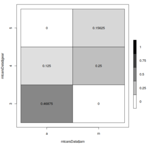
So I have created a function that produces a heat map for two categorical variables. It is called tableplot():

tableplot(mtcarsData$am,mtcarsData$gear)

It is based on table() function and uses the frequencies inside the table for the colours:

table(mtcarsData$am,mtcarsData$gear) / length(mtcarsData$am)

        3       4       5
a 0.46875 0.12500 0.00000
m 0.00000 0.25000 0.15625

The darker sectors mean that there is a higher concentration of values, while the white ones correspond to zeroes. So, in our example, we see that the majority of cars have automatic transmissions with three gears. Furthermore, the plot shows that there is some sort of relation between the two variables: the cars with automatic transmissions have the lower number of gears, while the ones with the manual have the higher number of gears (something we’ve already noticed in the previous subsection).

Association between the categorical and numerical variables

While Cramer’s V can also be used for the measurement of association between the variables in different scales, there are better instruments. For example, some analysts recommend using intraclass correlation coefficient when measuring the relation between the numerical and categorical variables. But there is a simpler option, which involves calculating the coefficient of multiple correlation between the variables. This is implemented in mcor() function of greybox. The `y` variable should be numerical, while `x` can be of any type. What the function then does is expands all the factors and runs a regression via .lm.fit() function, returning the square root of the coefficient of determination. If the variables are linearly related, then the returned value will be close to one. Otherwise it will be closet to zero. The function also returns the F statistics from the regression, the associated p-value and the number of degrees of freedom (the hypothesis is formulated similarly to cramer() function).

Here’s how it works:

mcor(mtcarsData$am,mtcarsData$mpg)

Multiple correlations value: 0.5998
F-statistics = 16.8603, df: 1, df resid: 30, p-value: 3e-04

In this example, the simple linear regression of mpg from the set of dummies is constructed, and we can conclude that there is a linear relation between the variables, and that this relation is statistically significant.

Association between several variables

Measures of association

When you deal with datasets (i.e. data frames or matrices), then you can use cor() function in order to calculate the correlation coefficients between the variables in the data. But when you have a mixture of numerical and categorical variables, the situation becomes more difficult, as the correlation does not make sense for the latter. This motivated me to create a function that uses either cor(), or cramer(), or mcor() functions depending on the types of data (see discussions of cramer() and mcor() above). The function is called association() or assoc() and returns three matrices: the values of the measures of association, their p-values and the types of the functions used between the variables. Here’s an example:

assocValues <- assoc(mtcarsData)
print(assocValues,digits=2)

 Associations: 
 values:
        mpg  cyl  disp    hp  drat    wt  qsec   vs   am gear carb
 mpg   1.00 0.86 -0.85 -0.78  0.68 -0.87  0.42 0.66 0.60 0.66 0.67
 cyl   0.86 1.00  0.92  0.84  0.70  0.78  0.59 0.82 0.52 0.53 0.62
 disp -0.85 0.92  1.00  0.79 -0.71  0.89 -0.43 0.71 0.59 0.77 0.56
 hp   -0.78 0.84  0.79  1.00 -0.45  0.66 -0.71 0.72 0.24 0.66 0.79
 drat  0.68 0.70 -0.71 -0.45  1.00 -0.71  0.09 0.44 0.71 0.83 0.33
 wt   -0.87 0.78  0.89  0.66 -0.71  1.00 -0.17 0.55 0.69 0.66 0.61
 qsec  0.42 0.59 -0.43 -0.71  0.09 -0.17  1.00 0.74 0.23 0.63 0.67
 vs    0.66 0.82  0.71  0.72  0.44  0.55  0.74 1.00 0.10 0.62 0.69
 am    0.60 0.52  0.59  0.24  0.71  0.69  0.23 0.10 1.00 0.81 0.44
 gear  0.66 0.53  0.77  0.66  0.83  0.66  0.63 0.62 0.81 1.00 0.51
 carb  0.67 0.62  0.56  0.79  0.33  0.61  0.67 0.69 0.44 0.51 1.00
 
 p-values:
       mpg  cyl disp   hp drat   wt qsec   vs   am gear carb
 mpg  1.00 0.00 0.00 0.00 0.00 0.00 0.02 0.00 0.00 0.00 0.01
 cyl  0.00 1.00 0.00 0.00 0.00 0.00 0.00 0.00 0.01 0.00 0.01
 disp 0.00 0.00 1.00 0.00 0.00 0.00 0.01 0.00 0.00 0.00 0.07
 hp   0.00 0.00 0.00 1.00 0.01 0.00 0.00 0.00 0.18 0.00 0.00
 drat 0.00 0.00 0.00 0.01 1.00 0.00 0.62 0.01 0.00 0.00 0.66
 wt   0.00 0.00 0.00 0.00 0.00 1.00 0.34 0.00 0.00 0.00 0.02
 qsec 0.02 0.00 0.01 0.00 0.62 0.34 1.00 0.00 0.21 0.00 0.01
 vs   0.00 0.00 0.00 0.00 0.01 0.00 0.00 1.00 0.56 0.00 0.01
 am   0.00 0.01 0.00 0.18 0.00 0.00 0.21 0.56 1.00 0.00 0.28
 gear 0.00 0.00 0.00 0.00 0.00 0.00 0.00 0.00 0.00 1.00 0.09
 carb 0.01 0.01 0.07 0.00 0.66 0.02 0.01 0.01 0.28 0.09 1.00
 
 types:
      mpg    cyl      disp   hp     drat   wt     qsec   vs       am      
 mpg  "none" "mcor"   "cor"  "cor"  "cor"  "cor"  "cor"  "mcor"   "mcor"  
 cyl  "mcor" "none"   "mcor" "mcor" "mcor" "mcor" "mcor" "cramer" "cramer"
 disp "cor"  "mcor"   "none" "cor"  "cor"  "cor"  "cor"  "mcor"   "mcor"  
 hp   "cor"  "mcor"   "cor"  "none" "cor"  "cor"  "cor"  "mcor"   "mcor"  
 drat "cor"  "mcor"   "cor"  "cor"  "none" "cor"  "cor"  "mcor"   "mcor"  
 wt   "cor"  "mcor"   "cor"  "cor"  "cor"  "none" "cor"  "mcor"   "mcor"  
 qsec "cor"  "mcor"   "cor"  "cor"  "cor"  "cor"  "none" "mcor"   "mcor"  
 vs   "mcor" "cramer" "mcor" "mcor" "mcor" "mcor" "mcor" "none"   "cramer"
 am   "mcor" "cramer" "mcor" "mcor" "mcor" "mcor" "mcor" "cramer" "none"  
 gear "mcor" "cramer" "mcor" "mcor" "mcor" "mcor" "mcor" "cramer" "cramer"
 carb "mcor" "cramer" "mcor" "mcor" "mcor" "mcor" "mcor" "cramer" "cramer"
      gear     carb    
 mpg  "mcor"   "mcor"  
 cyl  "cramer" "cramer"
 disp "mcor"   "mcor"  
 hp   "mcor"   "mcor"  
 drat "mcor"   "mcor"  
 wt   "mcor"   "mcor"  
 qsec "mcor"   "mcor"  
 vs   "cramer" "cramer"
 am   "cramer" "cramer"
 gear "none"   "cramer"
 carb "cramer" "none"

One thing to note is that the function considers numerical variables as categorical, when they only have up to 10 unique values. This is useful, for example, in case of number of `gears` in the dataset.

Plots of association between several variables

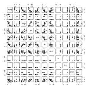
Similarly to the problem with cor(), scatterplot matrix (produced using plot()) is not meaningful in case of a mixture of variables:

plot(mtcarsData)

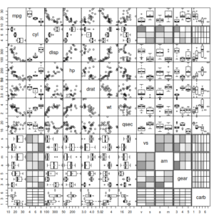
It makes sense to use scatterplot in case of numeric variables, tableplot() in case of categorical and boxplot() in case of a mixture. So, there is the function spread() in greybox that creates something more meaningful. It uses the same algorithm as assoc() function, but produces plots instead of calculating measures of association. So, `gear` will be considered as categorical and the function will produce either boxplot() or tableplot(), when plotting it against other variables.

Here’s an example:

spread(mtcarsData)

This plot demonstrates, for example, that the number of carburetors influences fuel consumption (something that we could not have spotted in the case of plot()). Notice also, that the number of gears influences the fuel consumption in a non-linear relation as well. So constructing the model with dummy variables for the number of gears might be a reasonable thing to do.

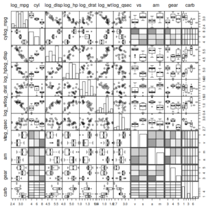
The function also has the parameter `log`, which will transform all the numerical variables using logarithms, which is handy, when you suspect the non-linear relation between the variables. Finally, there is a parameter `histogram`, which will plot either histograms, or barplots on the diagonal.

spread(mtcarsData, histograms=TRUE, log=TRUE)

The plot demonstrates that the `disp` has a strong non-linear relation with `mpg`, and, similarly, `drat` and `hp` also influence `mpg` in a non-linear fashion.

Regression diagnostics

One of the problems of linear regression that can be diagnosed prior to the model construction is multicollinearity. The conventional way of doing this diagnostics is via calculating the variance inflation factor (VIF) after constructing the model. However, VIF is not easy to interpret, because it lies in \((1,\infty)\). Coefficients of determination from the linear regression models of explanatory variables are easier to interpret and work with. If such a coefficient is equal to one, then there are some perfectly correlated explanatory variables in the dataset. If it is equal to zero, then they are not linearly related.

There is a function determination() or determ() in greybox that returns the set of coefficients of determination for the explanatory variables. The good thing is that this can be done before constructing any model. In our example, the first column, `mpg` is the response variable, so we can diagnose the multicollinearity the following way:

determination(mtcarsData[,-1])

       cyl      disp        hp      drat        wt      qsec        vs 
 0.9349544 0.9537470 0.8982917 0.7036703 0.9340582 0.8671619 0.8017720 
        am      gear      carb 
 0.7924392 0.8133441 0.8735577

As we can see from the output above, `disp` is the most linearly related with the variables, so including it in the model might cause the multicollinearity, which will decrease the efficiency of the estimates of parameters.