UPDATE: Starting from the v2.5.1 the cfType parameter has been renamed into loss. This post has been updated since then in order to include the more recent name.

A bit about estimates of parameters

Hi everyone! Today I want to tell you about parameters estimation of smooth functions. But before going into details, there are several things that I want to note. In this post we will discuss bias, efficiency and consistency of estimates of parameters, so I will use phrases like “efficient estimator”, implying that we are talking about some optimisation mechanism that gives efficient estimates of parameters. It is probably not obvious for people without statistical background to understand what the hell is going on and why we should care, so I decided to give a brief explanation. Although there are strict statistical definitions of the aforementioned terms (you can easily find them in Wikipedia or anywhere else), I do not want to copy-paste them here, because there are only a couple of important points worth mentioning in our context. So, let’s get started.

Bias refers to the expected difference between the estimated value of parameter (on a specific sample) and the “true” one. Having unbiased estimates of parameters is important because they should lead to more accurate forecasts (at least in theory). For example, if the estimated parameter is equal to zero, while in fact it should be 0.5, then the model would not take the provided information into account correctly and as a result will produce less accurate point forecasts and incorrect prediction intervals. In inventory this may mean that we constantly order 100 units less than needed only because the parameter is lower than it should be.

Efficiency means that if the sample size increases, then the estimated parameters will not change substantially, they will vary in a narrow range (variance of estimates will be small). In the case with inefficient estimates the increase of sample size from 50 to 51 observations may lead to the change of a parameter from 0.1 to, let’s say, 10. This is bad because the values of parameters usually influence both point forecasts and prediction intervals. As a result the inventory decision may differ radically from day to day. For example, we may decide that we urgently need 1000 units of product on Monday, and order it just to realise on Tuesday that we only need 100. Obviously this is an exaggeration, but no one wants to deal with such an erratic stocking policy, so we need to have efficient estimates of parameters.

Consistency means that our estimates of parameters will get closer to the stable values (what statisticians would refer to as “true” values) with the increase of the sample size. This is important because in the opposite case estimates of parameters will diverge and become less and less realistic. This once again influences both point forecasts and prediction intervals, which will be less meaningful than they should have been. In a way consistency means that with the increase of the sample size the parameters will become more efficient and less biased. This in turn means that the more observations we have, the better. There is a prejudice in the world of practitioners that the situation in the market changes so fast that the old observations become useless very fast. As a result many companies just through away the old data. Although, in general the statement about the market changes is true, the forecasters tend to work with the models that take this into account (e.g. Exponential smoothing, ARIMA). These models adapt to the potential changes. So, we may benefit from the old data because it allows us getting more consistent estimates of parameters. Just keep in mind, that you can always remove the annoying bits of data but you can never un-throw away the data.

Having clarified these points, we can proceed to the topic of today’s post.

One-step-ahead estimators of smooth functions

We already know that the default estimator used for smooth functions is Mean Squared Error (for one step ahead forecast). If the residuals are distributed normally / log-normally, then the minimum of MSE gives estimates that also maximise the respective likelihood function. As a result the estimates of parameters become nice: consistent and efficient. It is also known in statistics that minimum of MSE gives mean estimates of the parameters, which means that MSE also produces unbiased estimates of parameters (if the model is specified correctly and bla-bla-bla). This works very well, when we deal with symmetric distributions of random variables. But it may perform poorly otherwise.

In this post we will use the series N1823 for our examples:

library(Mcomp)
x <- ts(c(M3$N1823$x,M3$N1823$xx),frequency=frequency(M3$N1823$x))

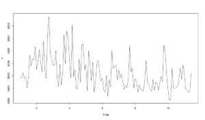
Plot the data in order to see what we have:

plot(x)

The data seems to have slight multiplicative seasonality, which changes over the time, but it is hard to say for sure. Anyway, in order to simplify things, we will apply an ETS(A,A,N) model to this data, so we can see how the different estimators behave. We will withhold 18 observations as it is usually done for monthly data in M3.

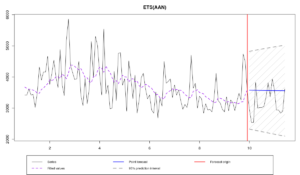
ourModel <- es(x,"AAN",silent=F,interval="p",h=18,holdout=T)

Here’s the output:

Time elapsed: 0.08 seconds
Model estimated: ETS(AAN)
Persistence vector g:
alpha  beta 
0.147 0.000 
Initial values were optimised.
5 parameters were estimated in the process
Residuals standard deviation: 629.249
Cost function type: MSE; Cost function value: 377623.069

Information criteria:
     AIC     AICc      BIC 
1703.389 1703.977 1716.800 
95% parametric prediction intervals were constructed
100% of values are in the prediction interval
Forecast errors:
MPE: -14%; Bias: -74.1%; MAPE: 16.8%; SMAPE: 15.1%
MASE: 0.855; sMAE: 13.4%; RelMAE: 1.047; sMSE: 2.4%

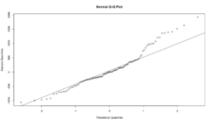
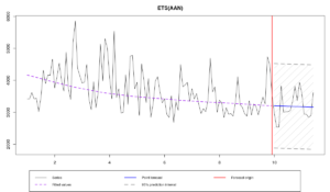
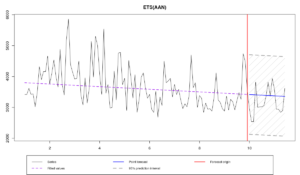
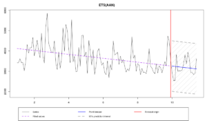
It is hard to make any reasonable conclusions from the graph and the output, but it seems that we slightly overforecast the data. At least the prediction interval covers all the values in the holdout. Relative MAE is equal to 1.047, which means that the model produced forecasts less accurate than Naive. Let’s have a look at the residuals:

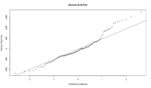
qqnorm(resid(ourModel))
qqline(resid(ourModel))

The residuals of this model do not look normal, a lot of empirical quantiles a far from the theoretical ones. If we conduct Shapiro-Wilk test, then we will have to reject the hypothesis of normality for the residuals on 5%:

shapiro.test(resid(ourModel))
> p-value = 0.001223

This may indicate that other estimators may do a better job. And there is a magical parameter loss in the smooth functions which allows to estimate models differently. It controls what to use and how to use it. You can select the following estimators instead of MSE:

• MAE – Mean Absolute Error:

\begin{equation} \label{eq:MAE}
\text{MAE} = \frac{1}{T} \sum_{t=1}^T |e_{t+1}|
\end{equation}

The minimum of MAE gives median estimates of the parameters. MAE is considered to be a more robust estimator than MSE. If you have asymmetric distribution, give MAE a try. It gives consistent, but not efficient estimates of parameters. Asymptotically, if the distribution of the residuals is normal, the estimators of MAE converge to the estimators of MSE (which follows from the connection between mean and median of normal distribution). Also, the minimum of MAE corresponds to the maximum of the likelihood of Laplace distribution (and the functions of the package use this property for the inference).

Let’s see what happens with the same model, on the same data when we use MAE:

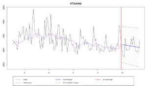
ourModel <- es(x,"AAN",silent=F,interval="p",h=18,holdout=T,loss="MAE")

Time elapsed: 0.09 seconds
Model estimated: ETS(AAN)
Persistence vector g:
alpha  beta 
0.101 0.000 
Initial values were optimised.
5 parameters were estimated in the process
Residuals standard deviation: 636.546
Cost function type: MAE; Cost function value: 462.675

Information criteria:
     AIC     AICc      BIC 
1705.879 1706.468 1719.290 
95% parametric prediction intervals were constructed
100% of values are in the prediction interval
Forecast errors:
MPE: -5.1%; Bias: -32.1%; MAPE: 12.9%; SMAPE: 12.4%
MASE: 0.688; sMAE: 10.7%; RelMAE: 0.842; sMSE: 1.5%

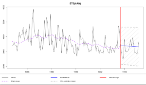
There are several things to note from the graph and the output. First, the smoothing parameter alpha is smaller than in the previous case. Second, Relative MAE is smaller than one, which means that model in this case outperformed Naive. Comparing this value with the one from the previous model, we can conclude that MAE worked well as an estimator of parameters for this data. Finally, the graph shows that point forecasts go through the middle of the holdout sample, which is reflected with lower values of error measures. The residuals are still not normally distributed, but this is expected, because they won't become normal just because we used a different estimator:

• HAM – Half Absolute Moment:

\begin{equation} \label{eq:HAM}
\text{HAM} = \frac{1}{T} \sum_{t=1}^T \sqrt{|e_{t+1}|}
\end{equation}
This is even more robust estimator than MAE. On count data its minimum corresponds to the mode of data. In case of continuous data the minimum of this estimator corresponds to something not yet well studied, between mode and median. The paper about this thing is currently in a draft stage, but you can already give it a try, if you want. This is also consistent, but not efficient estimator.

The same example, the same model, but HAM as an estimator:

ourModel <- es(x,"AAN",silent=F,interval="p",h=18,holdout=T,loss="HAM")

Time elapsed: 0.06 seconds
Model estimated: ETS(AAN)
Persistence vector g:
alpha  beta 
0.001 0.001 
Initial values were optimised.
5 parameters were estimated in the process
Residuals standard deviation: 666.439
Cost function type: HAM; Cost function value: 19.67

Information criteria:
     AIC     AICc      BIC 
1715.792 1716.381 1729.203 
95% parametric prediction intervals were constructed
100% of values are in the prediction interval
Forecast errors:
MPE: -1.7%; Bias: -14.1%; MAPE: 11.4%; SMAPE: 11.4%
MASE: 0.63; sMAE: 9.8%; RelMAE: 0.772; sMSE: 1.3%

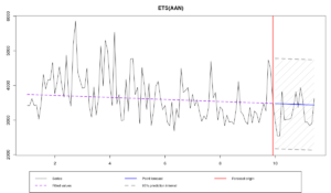
This estimator produced even more accurate forecasts in this example, forcing smoothing parameters to become close to zero. Note that the residuals standard deviation in case of HAM is larger than in case of MAE which in its turn is larger than in case of MSE. This means that one-step-ahead parametric and semiparametric prediction intervals will be wider in case of HAM than in case of MAE, than in case of MSE. However, taking that the smoothing parameters in the last model are close to zero, the multiple steps ahead prediction intervals of HAM may be narrower than the ones of MSE.

Finally, it is worth noting that the optimisation of models using different estimators takes different time. MSE is the slowest, while HAM is the fastest estimator. I don't have any detailed explanation of this, but this obviously happens because of the form of the cost functions surfaces. So if you are in a hurry and need to estimate something somehow, you can give HAM a try. Just remember that information criteria may become inapplicable in this case.

Multiple-steps-ahead estimators of smooth functions

While these three estimators above are calculated based on the one-step-ahead forecast error, the next three are based on multiple steps ahead estimators. They can be useful if you want to have a more stable and “conservative” model (a paper on this topic is currently in the final stage). Prior to v2.2.1 these estimators had different names, be aware!

• MSE\(_h\) - Mean Squared Error for h-steps ahead forecast:

\begin{equation} \label{eq:MSEh}
\text{MSE}_h = \frac{1}{T} \sum_{t=1}^T e_{t+h}^2
\end{equation}
The idea of this estimator is very simple: if you are interested in 5 steps ahead forecasts, then optimise over this horizon, not one-step-ahead. However, by using this estimator, we shrink the smoothing parameters towards zero, forcing the model to become closer to the deterministic and robust to outliers. This applies both to ETS and ARIMA, but the models behave slightly differently. The effect of shrinkage increases with the increase of \(h\). The forecasts accuracy may increase for that specific horizon, but it almost surely will decrease for all the other horizons. Keep in mind that this is in general not efficient and biased estimator with a much slower convergence to the true value than the one-step-ahead estimators. This estimator is eventually consistent, but it may need a very large sample to become one. This means that this estimator may result in values of parameters very close to zero even if they are not really needed for the data. I personally would advise using this thing on large samples (for instance, on high frequency data). By the way, Nikos Kourentzes, Rebecca Killick and I are working on a paper on that topic, so stay tuned.

Here’s what happens when we use this estimator:

ourModel <- es(x,"AAN",silent=F,interval="p",h=18,holdout=T,loss="MSEh")

Time elapsed: 0.24 seconds
Model estimated: ETS(AAN)
Persistence vector g:
alpha  beta 
    0     0 
Initial values were optimised.
5 parameters were estimated in the process
Residuals standard deviation: 657.781
Cost function type: MSEh; Cost function value: 550179.34

Information criteria:
     AIC     AICc      BIC 
30393.86 30404.45 30635.25 
95% parametric prediction intervals were constructed
100% of values are in the prediction interval
Forecast errors:
MPE: -10.4%; Bias: -62%; MAPE: 14.9%; SMAPE: 13.8%
MASE: 0.772; sMAE: 12.1%; RelMAE: 0.945; sMSE: 1.8%

As you can see, the smoothing parameters are now equal to zero, which gives us the straight line going through all the data. If we had 1008 observations instead of 108, the parameters would not be shrunk to zero, because the model would need to adapt to changes in order to minimise the respective cost function.

• TMSE - Trace Mean Squared Error:

The need for having a specific 5 steps ahead forecast is not common, so it makes sense to work with something that deals with one to h steps ahead:
\begin{equation} \label{TMSE}
\text{TMSE} = \sum_{j=1}^h \frac{1}{T} \sum_{t=1}^T e_{t+j}^2
\end{equation}
This estimator is more reasonable than MSE\(_h\) because it takes into account all the errors from one to h-steps-ahead forecasts. This is a desired behaviour in inventory management, because we are not so much interested in how much we will sell tomorrow or next Monday, but rather how much we will sell starting from tomorrow till the next Monday. However, the variance of forecast errors h-steps-ahead is usually larger than the variance of one-step-ahead errors (because of the increasing uncertainty), which leads to the effect of “masking”: the latter is hidden behind the former. As a result if we use TMSE as the estimator, the final values are seriously influenced by the long term errors than the short term ones (see Taieb and Atiya, 2015 paper). This estimator is not recommended if short-term forecasts are more important than long term ones. Plus, this is still less efficient and more biased estimator than one-step-ahead estimators, with slow convergence to the true values, similar to MSE\(_h\), but slightly better.

This is what happens in our example:

ourModel <- es(x,"AAN",silent=F,interval="p",h=18,holdout=T,loss="TMSE")

Time elapsed: 0.2 seconds
Model estimated: ETS(AAN)
Persistence vector g:
alpha  beta 
0.075 0.000 
Initial values were optimised.
5 parameters were estimated in the process
Residuals standard deviation: 633.48
Cost function type: TMSE; Cost function value: 7477097.717

Information criteria:
     AIC     AICc      BIC 
30394.36 30404.94 30635.75 
95% parametric prediction intervals were constructed
100% of values are in the prediction interval
Forecast errors:
MPE: -7.5%; Bias: -48.9%; MAPE: 13.4%; SMAPE: 12.6%
MASE: 0.704; sMAE: 11%; RelMAE: 0.862; sMSE: 1.5%

Comparing the model estimated using TMSE with the same one estimated using MSE and MSE\(_h\), it is worth noting that the smoothing parameters in this model are greater than in case of MSE\(_h\), but less than in case of MSE. This demonstrates that there is a shrinkage effect in TMSE, forcing the parameters towards zero, but the inclusion of one-step-ahead errors makes model slightly more flexible than in case of MSE\(_h\). Still, it is advised to use this estimator on large samples, where the estimates of parameters become more efficient and less biased.

• GTMSE - Geometric Trace Mean Squared Error:

This is similar to TMSE, but derived from the so called Trace Forecast Likelihood (which I may discuss at some point in one of the future posts). The idea here is to take logarithms of each MSE\(_j\) and then sum them up:
\begin{equation} \label{eq:GTMSE}
\text{GTMSE} = \sum_{j=1}^h \log \left( \frac{1}{T} \sum_{t=1}^T e_{t+j}^2 \right)
\end{equation}
Logarithms make variances of errors on several steps ahead closer to each other. For example, if the variance of one-step-ahead error is equal to 100 and the variance of 10 steps ahead error is equal to 1000, then their logarithms will be 4.6 and 6.9 respectively. As a result when GTMSE is used as an estimator, the model will take into account both short and long term errors. So this is a more balanced estimator of parameters than MSE\(_h\) and TMSE. This estimator is more efficient than both TMSE and MSE\(_j\) because of the log-scale and converges to true values faster than the previous two, but still can be biased on small samples.

ourModel <- es(x,"AAN",silent=F,interval="p",h=18,holdout=T,loss="GTMSE")

Time elapsed: 0.18 seconds
Model estimated: ETS(AAN)
Persistence vector g:
alpha  beta 
    0     0 
Initial values were optimised.
5 parameters were estimated in the process
Residuals standard deviation: 649.253
Cost function type: GTMSE; Cost function value: 232.419

Information criteria:
     AIC     AICc      BIC 
30402.77 30413.36 30644.16 
95% parametric prediction intervals were constructed
100% of values are in the prediction interval
Forecast errors:
MPE: -8.2%; Bias: -53.8%; MAPE: 13.8%; SMAPE: 12.9%
MASE: 0.72; sMAE: 11.3%; RelMAE: 0.882; sMSE: 1.6%

In our example GTMSE shrinks both smoothing parameters towards zero and makes the model deterministic, which corresponds to MSE\(_h\). However the initial values are slightly different, which leads to slightly different forecasts. Once again, it is advised to use this estimator on large samples.

Keep in mind that all those multiple steps ahead estimators take more time for the calculation, because the model needs to produce h-steps-ahead forecasts from each observation in sample.

• Analytical multiple steps ahead estimators.

There is also a non-documented feature in smooth functions (currently available only for pure additive models) – analytical versions of multiple steps ahead estimators. In order to use it, we need to add “a” in front of the desired estimator: aMSE\(_h\), aTMSE, aGTMSE. In this case only one-step-ahead forecast error is produced and after that the structure of the applied state-space model is used in order to reconstruct multiple steps ahead estimators. This feature is useful if you want to use the multiple steps ahead estimator on small samples, where the multi-steps errors cannot be calculated appropriately. It is also useful in cases of large samples, when the time of estimation is important.

These estimators have similar properties to their empirical counterparts, but work faster and are based on asymptotic properties. Here is an example of analytical MSE\(_h\) estimator:

ourModel <- es(x,"AAN",silent=F,interval="p",h=18,holdout=T,loss="aMSEh")

Time elapsed: 0.11 seconds
Model estimated: ETS(AAN)
Persistence vector g:
alpha  beta 
    0     0 
Initial values were optimised.
5 parameters were estimated in the process
Residuals standard deviation: 627.818
Cost function type: aMSEh; Cost function value: 375907.976

Information criteria:
     AIC     AICc      BIC 
30652.15 30662.74 30893.55 
95% parametric prediction intervals were constructed
100% of values are in the prediction interval
Forecast errors:
MPE: -1.9%; Bias: -14.6%; MAPE: 11.7%; SMAPE: 11.6%
MASE: 0.643; sMAE: 10%; RelMAE: 0.787; sMSE: 1.3%

The resulting smoothing parameters are shrunk towards zero, similar to MSE\(_h\), but the initial values are slightly different, which leads to different forecasts. Note that the time elapsed in this case is 0.11 seconds instead of 0.24 as in MSE\(_h\). The difference in time may increase with the increase of sample size and forecasting horizon.

• Similar to MSE, there are empirical multi-step MAE and HAM in smooth functions (e.g. MAE\(_h\) and THAM). However, they are currently implemented mainly “because I can” and for fun, so I cannot give you any recommendations about them.

• Starting from v2.4.0, a new estimator was introduced, "Mean Squared Cumulative Error" - MSCE, which may be useful in cases, when the cumulative demand is of the interest rather than point or trace ones.

Conclusions

Now that we discussed all the possible estimators that you can use with smooth, you are most probably confused and completely lost. The question that may naturally appear after you have read this post is “What should I do?” Frankly speaking, I cannot give you appropriate answer and a set of universal recommendations, because this is still under-researched problem. However, I have some advice.

First, Nikos Kourentzes and Juan Ramon Trapero found that in case of high frequency data (they used solar irradiation data) using MSE\(_h\) and TMSE leads to the increase in forecasting accuracy in comparison with the conventional MSE. However in order to achieve good accuracy in case of MSE\(_h\), you need to estimate \(h\) separate models, while with TMSE you need to estimate only one. So, TMSE is faster than MSE\(_h\), but at the same time leads to at least as accurate forecasts as in case of MSE\(_h\) for all the steps from 1 to h.

Second, if you have asymmetrically distributed residuals in the model after using MSE, give MAE or HAM a try – they may improve your model and its accuracy.

Third, analytical counterparts of multi-step estimators can be useful in one of the two situations: 1. When you deal with very large samples (e.g. high frequency data), want to use advanced estimation methods, but want them to work fast. 2. When you work with small sample, but want to use the properties of these estimators anyway.

Finally, don’t use MSE\(_h\), TMSE and GTMSE if you are interested in the values of parameters of models – they will almost surely be inefficient and biased. This applies to both ETS and ARIMA models, which will become close to their deterministic counterparts in this case. Use conventional MSE instead.