


Have you heard about the recursive vs direct forecasts? There’s literature about them in the areas of both ML and statistics. What’s so special about them? Here is a short post.
The term “recursive” forecasting refers to the approach, when we produce one-step-ahead forecast first, then use it to produce two-steps-ahead, three-steps-ahead, and so on. This process is iterative, fitting the model to the data based on one-step-ahead forecasts, starting from the first observation to the last in the sample. This is the default approach for all the standard dynamic models for forecasting, such as ARIMA or ETS.
The “direct” forecasting means producing a specific h-steps-ahead forecast (e.g., 12 months ahead), skipping intermediate steps. To do this, when fitting the model, we calculate the error between the one-step-ahead forecast and the actual value h steps ahead. This changes how we estimate the model, as our loss function is now based on the h-steps-ahead forecast error, and our one-step-ahead forecast starts acting as the h-steps-ahead one. Because of that, our one-step-ahead forecast now acts as the h-steps-ahead one. This way we don’t need to produce forecasts recursively, but, if we need all forecasts between 1 and h steps ahead, we must fit h models.
Both strategies are shown in the following image:
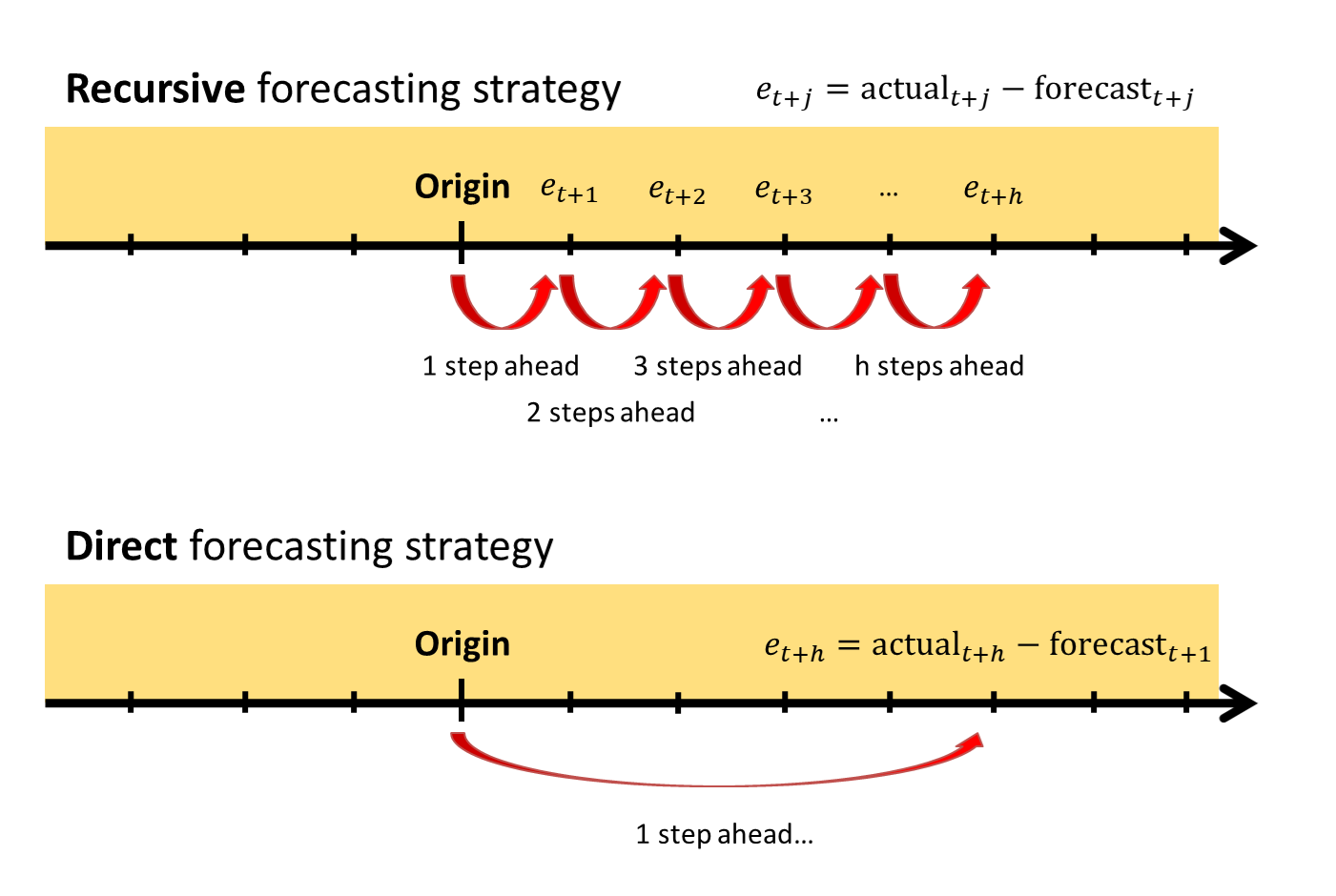
Recursive vs Direct forecasting strategies
The literature tells us that the direct forecasting strategy is equivalent to the so called multistep ahead loss function in model estimation (e.g. Chevillon, 2007). The standard “direct” forecasting strategy will give the same results as if we apply ARIMA/ETS to the data, produce h steps ahead recursive forecasts in-sample, starting from the first observation till the very last, and then minimise the Mean Squared h-steps-ahead forecast error (MSEh). This strategy has some advantages and disadvantages in comparison with the conventional one-step-ahead (see the introduction of our paper):
1. The specific h-steps-ahead forecast tends to be more accurate than in case of the standard estimation methods;
2. Although some papers show this isn’t universally true;
3. Parameter estimates tend to be less efficient than with one-step-ahead losses;
4. It’s more computationally expensive than standard estimators, especially for multiple-step forecasts.
So, there are accuracy benefits, but they come with a computational cost. Moreover, Kourentzes et al. (2020) found that the forecasting accuracy of MSEh was higher than the one of conventional loss functions, but this didn’t translate to better inventory performance.
Still, it wasn’t clear why this strategy is better, and we showed that applying MSEh to a dynamic model regularises its parameters. In ETS, this leads to parameters shrinkage toward zero proportionally to the forecast horizon used in the loss, making models more conservative and “slow.”
This is also discussed in Section 11.3 of ADAM.