Good news everyone! The future of statistical forecasting is finally here :). Have you ever struggled with ETS and needed explanatory variables? Have you ever needed to unite ARIMA and ETS? Have you ever needed to deal with all those zeroes in the data? What about the data with multiple seasonalities? All of this and more can now be solved by adam() function from smooth v3.0.1 package for R (on its way to CRAN now). ADAM stands for “Augmented Dynamic Adaptive Model” (I will talk about it in the next CMAF Friday Forecasting Talk on 15th January). Now, what is ADAM? Well, something like this:

The Creation of ADAM by Arne Niklas Jansson with my adaptation
ADAM is the next step in time series analysis and forecasting. Remember exponential smoothing and functions like es() and ets()? Remember ARIMA and functions like arima(), ssarima(), msarima() etc? Remember your favourite linear regression function, e.g. lm(), glm() or alm()? Well, now these three models are implemented in a unified framework. Now you can have exponential smoothing with ARIMA elements and explanatory variables in one box: adam(). You can do ETS components and ARIMA orders selection, together with explanatory variables selection in one go. You can estimate ETS / ARIMA / regression using either likelihood of a selected distribution or using conventional losses like MSE, or even using your own custom loss. You can tune parameters of optimiser and experiment with initialisation and estimation of the model. The function can deal with multiple seasonalities and with intermittent data in one place. In fact, there are so many features that it is just easier to list the major of them:
- ETS;
- ARIMA;
- Regression;
- TVP regression;
- Combination of (1), (2) and either (3), or (4);
- Automatic selection / combination of states for ETS;
- Automatic orders selection for ARIMA;
- Variables selection for regression part;
- Normal and non-normal distributions;
- Automatic selection of most suitable distributions;
- Advanced and custom loss functions;
- Multiple seasonality;
- Occurrence part of the model to handle zeroes in data (intermittent demand);
- Model diagnostics using plot() and other methods;
- Confidence intervals for parameters of models;
- Automatic outliers detection;
- Handling missing data;
- Fine tuning of persistence vector (smoothing parameters);
- Fine tuning of initial values of the state vector (e.g. level / trend / seasonality / ARIMA components / regression parameters);
- Two initialisation options (optimal / backcasting);
- Provided ARMA parameters;
- Fine tuning of optimiser (select algorithm and convergence criteria);
- …
All of this is based on the Single Source of Error state space model, which makes ETS, ARIMA and regression directly comparable via information criteria and opens a variety of modelling and forecasting possibilities. In addition, the code is much more efficient than the code of already existing smooth functions, so hopefully this will be a convenient function to use. I do not promise that everything will work 100% efficiently from scratch, because this is a new function, which implies that inevitably there are bugs and there is a room for improvement. But I intent to continue working on it, improving it further, based on the provided feedback (you can submit an issue on github if you have ideas).
Keep in mind that starting from smooth v3.0.0 I will not be introducing new features in es(), ssarima() and other conventional functions for univariate variables in smooth – I will only fix bugs in them and possibly optimise some parts of the code, but there will be no innovations in them, given that the main focus from now on will be on adam(). To that extent, I have removed some experimental and not fully developed parameters from those functions (e.g. occurrence, oesmodel, updateX, persistenceX and transitionX).
Now, I realise that ADAM is something completely new and contains just too much information to cover in one post. As a result, I have started the work on an online textbook. This is work in progress, missing some chapters, but it already covers many important elements of ADAM. If you find any mistakes in the text or formulae, please, use the “Open Review” functionality in the textbook to give me feedback or send me a message. This will be highly appreciated, because, working on this alone, I am sure that I have made plenty of mistakes and typos.
Example in R
Finally, it would be boring just to announce things and leave it like that. So, I’ve decided to come up with an R experiments on M, M3 and tourism competitions data, similar to how I’ve done it in 2017, just to show how the function compares with the other conventional ones, measuring their accuracy and computational time:
After running this code, we will get the big array (7x5315x21), which would contain many different error measures for point forecasts and prediction intervals. We will not use all of them, but instead will extract MASE and RMSSE for point forecasts and Coverage, Range and sMIS for prediction intervals, together with computational time. Although it might be more informative to look at distributions of those variables, we will calculate mean and median values overall, just to get a feeling about the performance:
Means:
               MASE RMSSE Coverage Range  sMIS  Time
ADAM-ETS(ZZZ) 2.415 2.098    0.888 1.398 2.437 0.654
ADAM-ETS(ZXZ) 2.250 1.961    0.895 1.225 2.092 0.497
ADAM-ARIMA    2.551 2.203    0.862 0.968 3.098 5.990
ETS(ZXZ)      2.279 1.977    0.862 1.372 2.490 1.128
ETSHyndman    2.263 1.970    0.882 1.200 2.258 0.404
AutoSSARIMA   2.482 2.134    0.801 0.780 3.335 1.700
AutoARIMA     2.303 1.989    0.834 0.805 3.013 1.385

Medians:
               MASE RMSSE Range  sMIS  Time
ADAM-ETS(ZZZ) 1.362 1.215 0.671 0.917 0.396
ADAM-ETS(ZXZ) 1.327 1.184 0.675 0.909 0.310
ADAM-ARIMA    1.476 1.300 0.769 1.006 3.525
ETS(ZXZ)      1.335 1.198 0.616 0.931 0.551
ETSHyndman    1.323 1.181 0.653 0.925 0.164
AutoSSARIMA   1.419 1.271 0.577 0.988 0.909
AutoARIMA     1.310 1.182 0.609 0.881 0.322
Some things to note from this:
- ADAM ETS(ZXZ) is the most accurate model in terms of mean MASE and RMSSE, it has the coverage closest to 95% (although none of the models achieved the nominal value because of the fundamental underestimation of uncertainty) and has the lowest sMIS, implying that it did better than the other functions in terms of prediction intervals;
- The ETS(ZZZ) did worse than ETS(ZXZ) because the latter considers the multiplicative trend, which sometimes becomes unstable, producing exploding trajectories;
- ADAM ARIMA is not performing well yet, because of the implemented order selection algorithm and it was the slowest function of all. I plan to improve it in future releases of the function;
- While ADAM ETS(ZXZ) did not beat ETS from forecast package in terms of computational time, it was faster than the other functions;
- When it comes to medians,
auto.arima(),ets()andauto.ssarima()seem to be doing better than ADAM, but not by a large margin.
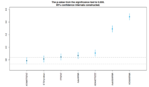
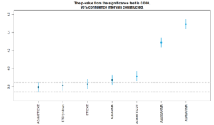
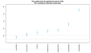
In order to see if the performance of functions is statistically different, we run the RMCB test for MASE, RMSSE and MIS. Note that RMCB compares the median performance of functions. Here is the R code:
And here are the figures that we get by running that code
As we can see from the two figures above, ADAM-ETS(Z,X,Z) performs better than the other functions, although statistically not different than ETS implemented in es() and ets() functions. ADAM-ARIMA is the worst performing function for the moment, as we have already noticed in the previous analysis. The ranking is similar for both MASE and RMSSE.
And here is the sMIS plot:
When it comes to sMIS, the leader in terms of medians is auto.arima(), doing quite similar to ets(), but this is mainly because they have lower ranges, incidentally resulting in lower than needed coverage (as seen from the summary performance above). ADAM-ETS does similar to ets() and es() in this aspect (the intervals of the three intersect).
Obviously, we could provide more detailed analysis of performance of functions on different types of data and see, how they compare in each category, but the aim of this post is just to demonstrate how the new function works, I do not have intent to investigate this in detail.
Finally, I will present ADAM with several case studies in CMAF Friday Forecasting Talk on 15th January. If you are interested to hear more and have some questions, please register on MeetUp or via LinkedIn and join us online.


