17.3 Example in R
17.3.1 Example 1
To demonstrate how the scale model works, we will use the model that we constructed in Section 10.6 (we use Normal distribution for simplicity):
adamLocationSeat <- adam(SeatbeltsData, "MNM", h=12, holdout=TRUE,
                         formula=drivers~log(kms)+log(PetrolPrice)+law,
                         distribution="dnorm")
To see if the scale model is needed in this case, we will produce several diagnostics plots (Figure 17.1).
par(mfcol=c(2,1), mar=c(4,4,2,1))
plot(adamLocationSeat, which=c(4,8))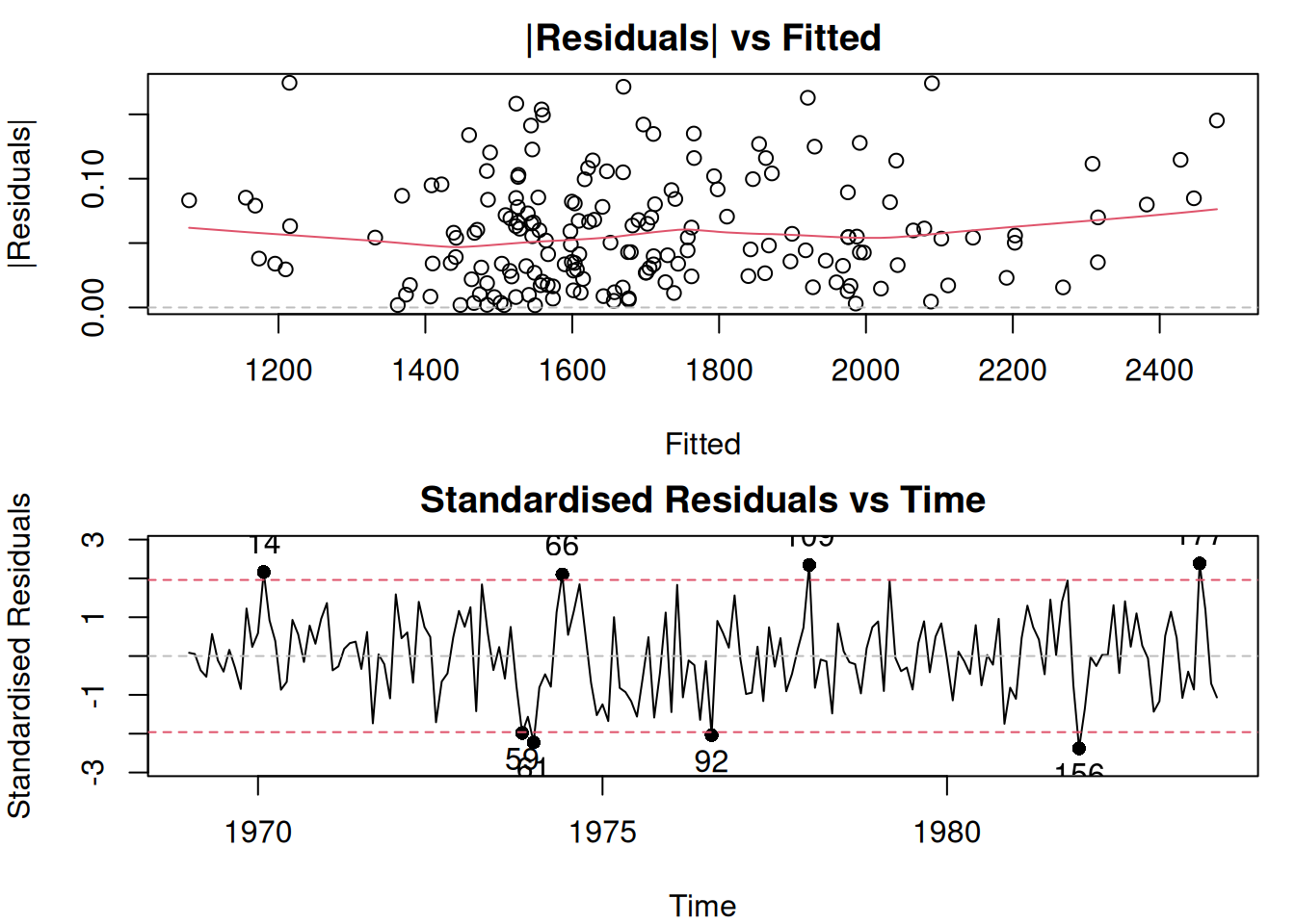
Figure 17.1: Diagnostic plots for the ETSX(M,N,M) model.
Figure 17.1 shows how the residuals change with: (1) change of fitted values, (2) change of time. The first plot shows that there might be a slight change in the variability of residuals, but it is not apparent. The second plot does not demonstrate any significant changes in variance over time. To check the latter point more formally, we can also produce ACF and PACF of the squared residuals, thus trying to see if GARCH model is required:
par(mfcol=c(2,1), mar=c(4,4,2,1))
plot(adamLocationSeat, which=c(15,16))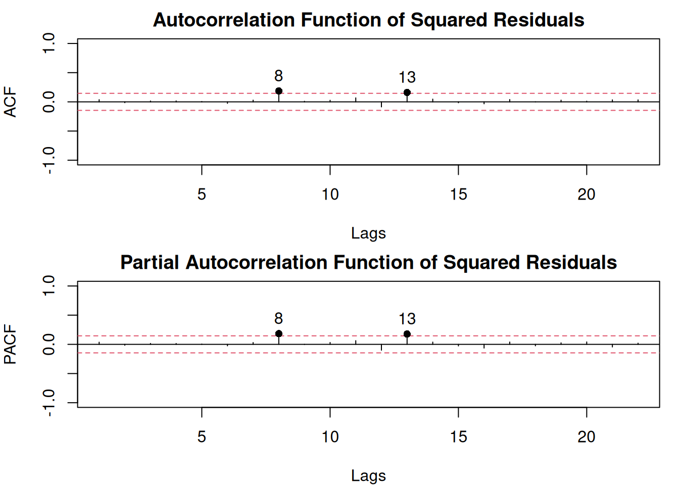
Figure 17.2: Diagnostic plots for the ETSX(M,N,M) model, continued.
In the plot of Figure 17.2, lag 8 is significant on both ACF and PACF and lag 13 is significant on PACF. We could introduce the dynamic elements in the scale model to remove this autocorrelation, however the lags 8 and 13 do not have any meaning from the problem point of view: it is difficult to motivate how a variance 8 months ago might impact the variance this month. Furthermore, the bounds in the plot have the 95% confidence level, which means that these coefficients could have become significant by chance. So, based on this simple analysis, we can conclude that there might be some factors impacting the variance of residuals, but it does not exhibit any obvious and meaningful GARCH-style dynamics. To investigate this further, we can plot explanatory variables vs the squared residuals (Figure 17.3).
spread(cbind(residSq=as.vector(resid(adamLocationSeat)^2),
             as.data.frame(SeatbeltsData)[1:180,-1]),
       lowess=TRUE)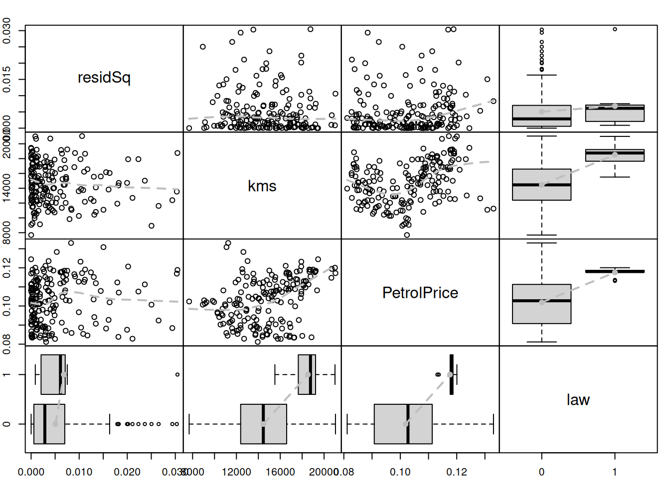
Figure 17.3: Spread plot for the ETSX(M,N,M) model.
One of the potentially alarming feature in the plot in Figure 17.3 is the slight change in variance for the variable law. The second one is a slight increase in the LOWESS line for squared residuals vs PetrolPrice. The kms variable does not demonstrate an apparent impact on the squared residuals. Based on this, we will investigate the potential effect of the law and petrol price on the scale of the model. We do that in an automated way, using the principles discussed in Section 15.3 via regressors="select" command:
adamScaleSeat <- sm(adamLocationSeat, model="NNN",
                    formula=drivers~law+PetrolPrice,
                    regressors="select")
## Warning: This type of model can only be applied to the data in logarithms.
## Amending the dataIn the code above, we fit a scale model to the already estimated location model ETSX(M,N,M). We switch off the ETS element in the scale model and introduce the explanatory variables law and PetrolPrice, asking the function to select the most appropriate one based on AICc. The function provides a warning that it will create a model in logarithms, which is what we want anyway. But looking at the output of the scale model, we notice that none of the variables have been selected by the function:
summary(adamScaleSeat)##
## Model estimated using sm.adam() function: Regression in logs
## Response variable: drivers
## Distribution used in the estimation: Normal
## Loss function type: likelihood; Loss function value: -418.9007
## Coefficients:
## Estimate Std. Error Lower 2.5% Upper 97.5%
## (Intercept) -6.5769 0.1416 -6.8563 -6.2974 *
##
## Error standard deviation: 1.9
## Sample size: 180
## Number of estimated parameters: 1
## Number of degrees of freedom: 179
## Information criteria:
## AIC AICc BIC BICc
## -835.8014 -835.7790 -832.6085 -832.5501This means that the explanatory variables do not add value to the fit and should not be included in the scale model. As we can see, selection of variables in the scale model for ADAM can be done automatically without any additional external steps.
17.3.2 Example 2
The example in the previous Subsection shows how the analysis can be done for the scale model when explanatory variables are considered. To see how the scale model can be used in forecasting, we will consider another example, now with dynamic elements. For this example, I will use AirPassengers data and an automatically selected ETS model with Inverse Gaussian distribution (for demonstration purposes):
adamLocationAir <- adam(AirPassengers, h=10, holdout=TRUE,
                        distribution="dinvgauss")
The diagnostics of the model indicate that a time-varying scale might be required in this situation (see Figure 17.4) because the variance of the residuals seems to decrease in the period from 1954 – 1958.
plot(adamLocationAir, which=8)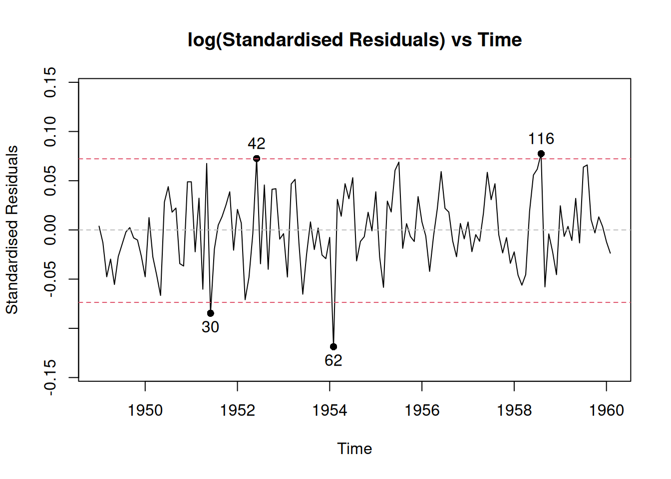
Figure 17.4: Diagnostics of the location model
To capture this change, we will ask the function to select the best ETS model for the scale and will not use any other elements:
adamScaleAir <- sm(adamLocationAir, model="YYY")The sm function accepts roughly the same set of parameters as adam() when applied to the adam class objects. So, you can experiment with other types of ETS/ARIMA models if you want. Here is what the function has selected automatically for the scale model:
summary(adamScaleAir)## Warning: Observed Fisher Information is not positive semi-definite, which means
## that the likelihood was not maximised properly. Consider reestimating the
## model, tuning the optimiser or using bootstrap via bootstrap=TRUE.##
## Model estimated using sm.adam() function: ETS(MNN)
## Response variable: AirPassengers
## Distribution used in the estimation: Inverse Gaussian
## Loss function type: likelihood; Loss function value: 474.332
## Coefficients:
## Estimate Std. Error Lower 2.5% Upper 97.5%
## alpha 0.0704 0.0569 0e+00 0.1828
## level 0.0021 0.0011 -1e-04 0.0043
##
## Error standard deviation: 1.41
## Sample size: 134
## Number of estimated parameters: 2
## Number of degrees of freedom: 132
## Information criteria:
## AIC AICc BIC BICc
## 952.6640 952.7556 958.4596 958.6840Remark. Information criteria in the summary of the scale model do not include the number of estimated parameters in the location part of the model, so they are not directly comparable with the ones from the initial model. So, to understand whether there is an improvement in comparison with the model with a fixed scale, we can implant the scale model in the location one and compare the new model with the initial one:
adamMerged <- implant(adamLocationAir, adamScaleAir)
c(AICc(adamLocationAir), AICc(adamMerged)) |>
         setNames(c("Location", "Merged"))
## Location Merged
## 991.4883 990.6118The output above shows that introducing the ETS(M,N,N) model for the scale has improved the ADAM, reducing the AICc.
Judging by the output, we see that the most suitable model for the location is ETS(M,N,N) with \(\alpha=0.0704\), which, as we discussed in Subsection 17.2, is equivalent to GARCH(1,1) with restricted parameters: \[\begin{equation*} \sigma_t^2 = 0.9296 \sigma_{t-1}^2 + 0.0704 \epsilon_{t-1}^2 . \end{equation*}\]
After implanting the scale in the model, we can access it via adamMerged$scale and extract the predicted scale via extractScale(adamMerged) command in R. The model fits the data in the following way (see Figure 17.5):
plot(adamMerged$scale, which=7)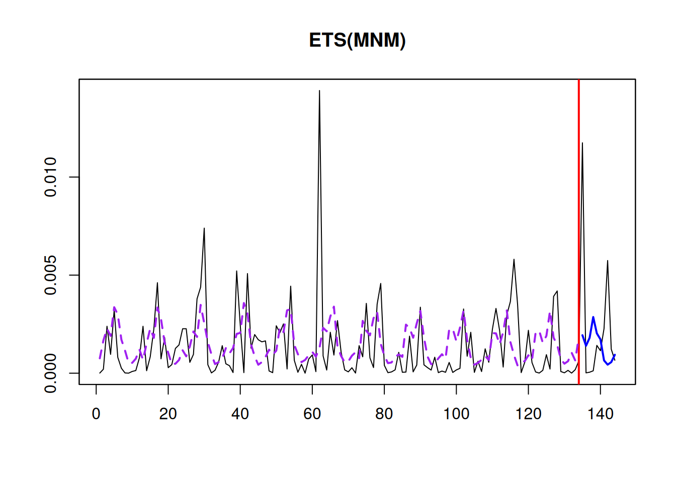
Figure 17.5: The fit of the scale model.
As can be seen from Figure 17.5, the scale changes over time, indeed decreasing in the middle of series and going slightly up at the end. The actual values in the holdout part can in general be ignored because they show the forecast errors several steps ahead for the whole holdout and are not directly comparable with the in-sample ones.
We can also do diagnostics of the merged model using the same principles as discussed in Chapter 14 – the function will automatically use the fitted values of scale where needed (see Figure 17.6).
par(mfcol=c(2,2), mar=c(4,4,2,1))
plot(adamMerged, which=c(2,6,8,7))
## Note that residuals diagnostics plots are produced for scale model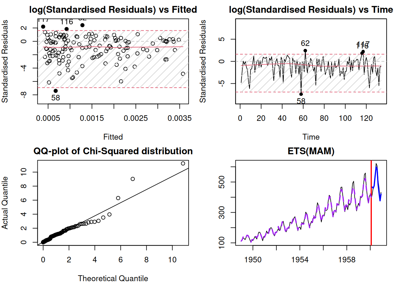
Figure 17.6: Diagnostics of the merged ADAM
Remark. In the case of a merged model, the plots that produce residuals will be done for the scale model rather than for the location (the plot function will produce a message on that), so plotting \(\eta_t\) instead of \(\epsilon_t\) (see discussion in Subsection 17.1.3 for the assumptions about the residual in this case).
Figure 17.6 demonstrates the diagnostics for the constructed model. Given that we used the Inverse Gaussian distribution, the \(\eta_t^2 \sim \chi^2(1)\), which is why the QQ-plot mentions the Chi-Squared distribution. We can see that the distribution has a shorter tail than expected, which means that the model might be missing some elements. However, the log(standardised Residuals) vs Fitted and vs Time do not demonstrate any obvious problems except for several potential outliers, which do not lie far away from the bounds and do not exheed 5% of the sample size in quantity. Those specific observations could be investigated to determine whether the model can be improved further. I leave this exercise to the reader.
Finally, if we want to produce forecasts from the scale model, we can use the same methods previously used for the location one (Figure 17.7).
forecast(adamMerged$scale,
         h=10, interval="prediction") |>
    plot()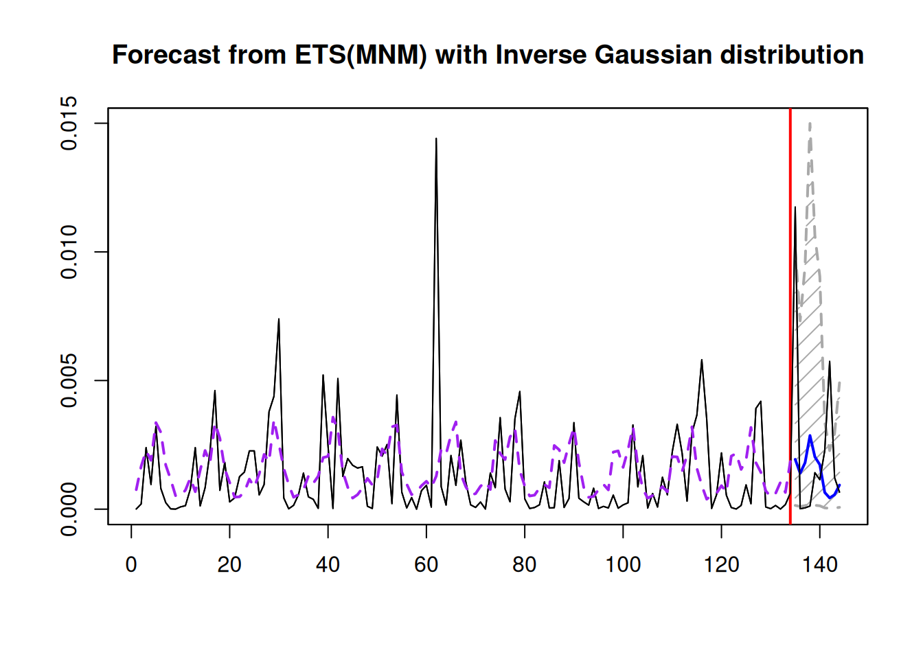
Figure 17.7: Forecast for the Scale model
The point forecast of the scale for the subsequent h observations can also be used to produce more appropriate prediction intervals for the merged model. This will be discussed in Chapter 18.