


At the end of June 2021, I released the greybox package version 1.0.0. This was a major release, introducing new functionality, but I did not have time to write a separate post about it because of the teaching and lack of free time. Finally, Christmas has arrived, and I could spend several hours preparing the post about it. In this post, I want to tell you about the new major feature in the greybox package.
Scale Model
The Scale Model is the regression-like model focusing on capturing the relation between the scale of distribution (for example, variance in Normal distribution) and a set of explanatory variables. It is implemented in sm() method in the greybox package. The motivation for this comes from GAMLSS, the Generalised Additive Model for Location, Scale and Shape. While I have decided not to bother with the “GAM” part of this (there are gam and gamlss packages in R that do that), I liked the idea of being able to predict the scale (for example, variance) of a distribution. This becomes especially useful when one suspects heteroscedasticity in the model but does not think that variable transformations are appropriate.
To understand what the function does, it is necessary first to discuss the underlying model. We will start the discussion with an example of a linear regression model with two explanatory variables, assuming Normally distributed residuals \(\xi_t\) with zero mean and a fixed variance \(\sigma^2\), \(\xi_t \sim \mathcal{N}(0,\sigma^2)\), which can be formulated as:
\begin{equation} \label{eq:model1}
y_t = \beta_0 + \beta_1 x_{1,t} + \beta_2 x_{2,t} + \xi_t ,
\end{equation}
where \(y_t\) is the response variable, \(x_{1,t}\) and \(x_{2,t}\) are the explanatory variables on observation \(t\), \(\beta_0\), \(\beta_1\) and \(\beta_2\) are the parameters of the model and \(\xi_t \sim \mathcal{N}\left(0, \sigma^2 \right)\). Recalling the basic properties of Normal distribution, we can rewrite the same model as a model with standard normal residuals \(\epsilon_t \sim \mathcal{N}\left(0, 1 \right)\) by inserting \(\xi_t = \sigma \epsilon_t\) in \eqref{eq:model1}:
\begin{equation} \label{eq:model2}
y_t = \beta_0 + \beta_1 x_{1,t} + \beta_2 x_{2,t} + \sigma \epsilon_t .
\end{equation}
Now if we suspect that the variance of the model might not be constant, we can substitute the standard deviation \(\sigma\) with some function, transforming the model into:
\begin{equation} \label{eq:model3}
y_t = \beta_0 + \beta_1 x_{1,t} + \beta_2 x_{2,t} + f\left(\gamma_0 + \gamma_2 x_{2,t} + \gamma_3 x_{3,t}\right) \epsilon_t ,
\end{equation}
where \(x_{2,t}\) and \(x_{3,t}\) are the explanatory variables (as you see, not necessarily the same as in the first part of the model) and \(\gamma_0\), \(\gamma_1\) and \(\gamma_2\) are the parameters of the scale part of the model. The idea here is that there is a regression model for the conditional mean of the distribution \(\beta_0 + \beta_1 x_{1,t} + \beta_2 x_{2,t}\), and that there is another one that will regulate the standard deviation via \(f\left(\gamma_0 + \gamma_2 x_{2,t} + \gamma_3 x_{3,t}\right)\). The main thing to keep in mind about the latter is that the function \(f(\cdot)\) needs to be strictly positive because the standard deviation cannot be zero or negative. The simplest way to guarantee this is to use exponent instead of \(f(\cdot)\). Furthermore, in our example with Normal distribution, the scale corresponds to the variance, so we should be introducing the model for variance: \(\sigma^2_t = \exp\left(\gamma_0 + \gamma_2 x_{2,t} + \gamma_3 x_{3,t}\right)\). This leads to the following model:
\begin{equation} \label{eq:model4}
y_t = \beta_0 + \beta_1 x_{1,t} + \beta_2 x_{2,t} + \sqrt{\exp\left(\gamma_0 + \gamma_2 x_{2,t} + \gamma_3 x_{3,t}\right)} \epsilon_t ,
\end{equation}
The model above would not only have the conditional mean depending on the values of explanatory variables (the conventional regression) but also the conditional variance, which would change depending on the values of variables. Note that this model assumes the linearity in the conditional mean: increase of \(x_{1,t}\) by one leads to the increase of \(y_t\) by \(\beta_1\) on average. At the same time, it assumes non-linearity in the variance: increase of \(x_{2,t}\) by one leads to the increase of variance by \(\exp(\gamma_2-1)\times 100\)%. If we want a non-linear change in the conditional mean, we can use a model in logarithms. Alternatively, we could assume a different distribution for the response variable \(y_t\). To understand how the latter would work, we need to represent the same model \eqref{eq:model4} in a more general form. For the Normal distribution, the same model \eqref{eq:model4} can be rewritten as:
\begin{equation} \label{eq:model5}
y_t \sim \mathcal{N}\left(\beta_0 + \beta_1 x_{1,t} + \beta_2 x_{2,t}, \exp\left(\gamma_0 + \gamma_2 x_{2,t} + \gamma_3 x_{3,t}\right)\right).
\end{equation}
This representation allows introducing scale model for many other distributions, such as Laplace, Generalised Normal, Gamma, Inverse Gaussian etc. All that we need to do in those cases is to substitute the distribution \(\mathcal{N}(\cdot)\) with a distribution of interest. The sm() function supports the same list of distributions as alm() (see the vignette for the function on CRAN or in R using the command vignette()). Each specific formula for scale would differ from one distribution to another, but the principles will be the same.
Demonstration in R
For demonstration purposes, we will use an example with artificial data, generated according to the model \eqref{eq:model4}:
xreg <- matrix(rnorm(300,10,3),100,3)
xreg <- cbind(1000-0.75*xreg[,1]+1.75*xreg[,2]+
              sqrt(exp(0.3+0.5*xreg[,2]-0.4*xreg[,3]))*rnorm(100,0,1),xreg)
colnames(xreg) <- c("y",paste0("x",c(1:3)))
The scatterplot of the generated data will look like this:
spread(xreg)
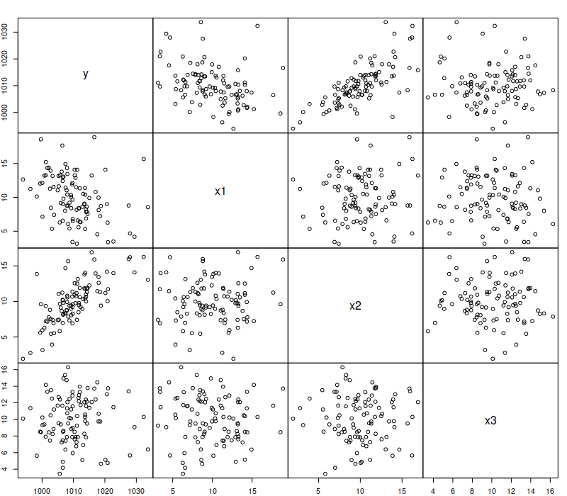
Scatterplot matrix for the generated data
We can then fit a model, specifying the location and scale parts of it in alm(). In this case, the alm() will call for sm() and will estimate both parts via likelihood maximisation. To make things closer to forecasting task, we will withhold the last 10 observations for the test set:
ourModel <- alm(y~x1+x2+x3, scale=~x2+x3, xreg, subset=c(1:90), distribution="dnorm")
The returned model contains both parts. The scale part of the model can be accessed via ourModel$scale. It is an object of class "scale", supporting several methods, such as
actuals(), residuals(), fitted(), summary() and plot() (and several other). Here how the summary of the model looks in my case:
summary(ourModel)
Response variable: y
Distribution used in the estimation: Normal
Loss function used in estimation: likelihood
Coefficients:
             Estimate Std. Error Lower 2.5% Upper 97.5%
(Intercept) 1000.2850     2.9698   994.3782   1006.1917 *
x1            -0.8350     0.1435    -1.1204     -0.5497 *
x2             1.8656     0.1714     1.5246      2.2065 *
x3            -0.0228     0.1776    -0.3761      0.3305

Coefficients for scale:
            Estimate Std. Error Lower 2.5% Upper 97.5%
(Intercept)   0.0436     0.7012    -1.3510      1.4382
x2            0.4705     0.0413     0.3883      0.5527 *
x3           -0.3355     0.0487    -0.4324     -0.2385 *

Error standard deviation: 4.52
Sample size: 90
Number of estimated parameters: 7
Number of degrees of freedom: 83
Information criteria:
     AIC     AICc      BIC     BICc
391.0191 392.3849 408.5177 411.5908
The summary above shows parameters for both parts of the model. They are not far from the ones used in the generation of the model, which indicates that the implemented model works as intended. The only issue here is that the standard errors in the location part of the model (first four coefficients) do not take the heteroscedasticity into account and thus are biased. The HAC standard errors are not yet implemented in alm()
As we see, the returned model contains both parts. The scale part of the model can be accessed via ourModel$scale. It is an object of class "scale", supporting several methods, such as
actuals(), residuals(), fitted(), summary() and plot() (and several other). Just to see the effect of scale model, here are the diagnostics plots for the original model (which returns the \(\xi_t\) residuals) and for the scale model (\(\epsilon_t\) residuals):
par(mfcol=c(1,2))
plot(ourModel, 5)
plot(ourModel, 5)
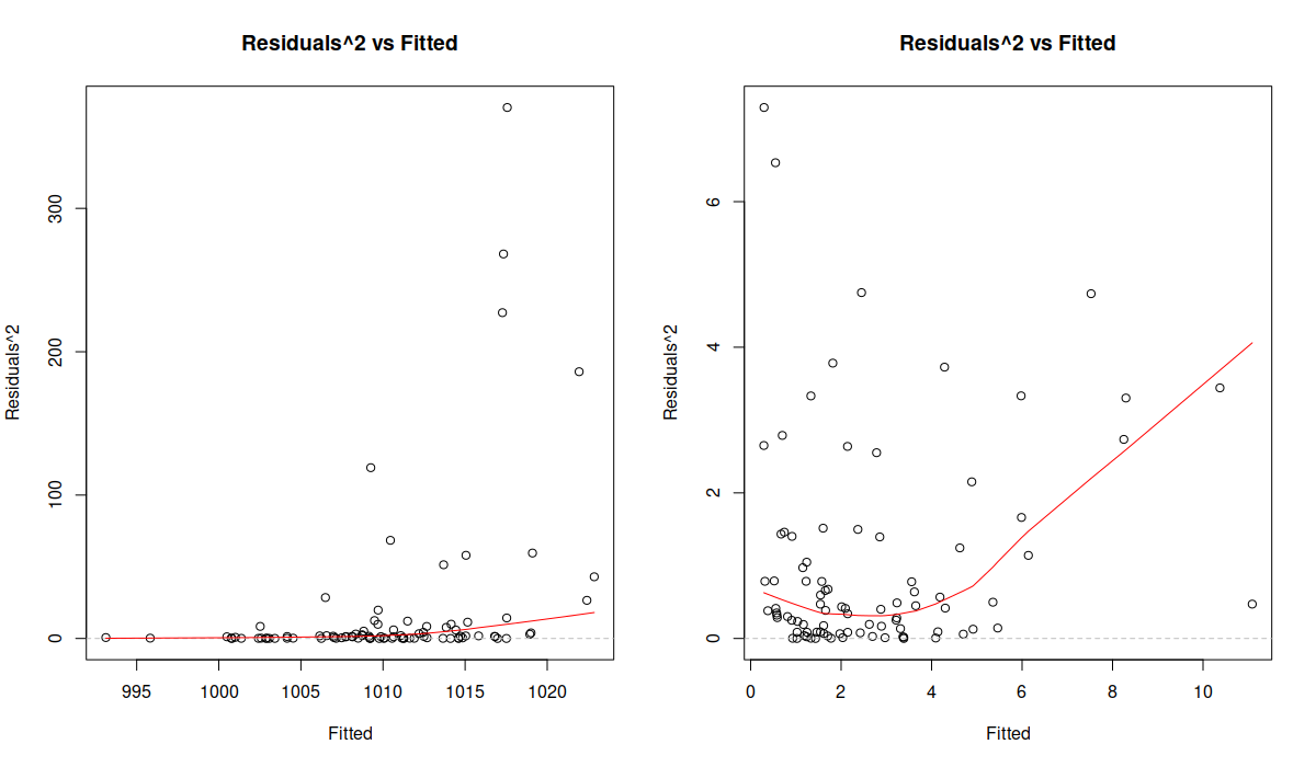
Diagnostics plots for sm
The Figure above shows squared residuals vs fitted values for the location (the plot on the left) and the scale (the plot on the right) models. The former is agnostic of the scale model and demonstrates that there is heteroscedasticity of residuals (the variance increases with the increase of the fitted values). The latter shows that the scale model managed to resolve the issue. While the LOWESS line demonstrates some non-linearity, the distribution of residuals conditional on fitted values looks random.
Finally, we can produce forecasts from such model, similarly to how it is done for any other model, estimated with alm():
ourForecast <- predict(ourModel,xreg[-c(1:90),],interval="pred")
plot(ourForecast)
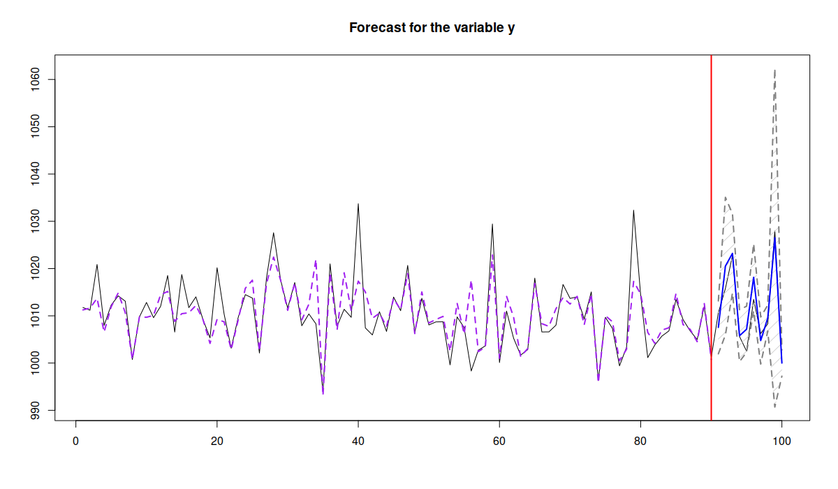
Forecast from the model
In this case, the function will first predict the scale part of the model, then it will use the predicted variance and the covariance matrix of parameters to calculate the prediction intervals, shown in Figure above. Given the independence of location and scale parts of the model, the conditional expectation (point forecast) will not change if we drop the scale model. It is all about variance.
Finally, if you do not want to use alm() function, you can use lm() instead and then apply the sm():
lmModel <- lm(y~x1+x2+x3, as.data.frame(xreg), subset=c(1:90))
smModel <- sm(lmModel, formula=~x2+x3, xreg)
In this case, the sm() will assume that the error term follows Normal distribution, and we will end up with two models that are not connected with each other (e.g., the predict() method applied to lmModel will not use predictions from the smModel). Nonetheless, we could still use all the R methods discussed above for the analysis of the smModel.
As a final word, the scale model is a new feature. While it already works, there might be bugs in it. If you find any, please let me know by submitting an issue on Github.
P.S.
There is a danger that greybox package will be soon removed from CRAN together with other 88 packages (including my smooth and legion) because the nloptr package that it relies on has not passed some of new checks recently introduced by CRAN. This is beyond my control, and I do not have time or power to influence this, but if this happens, you might need to switch to the installation from GitHub via remotes package, using the command:
remotes::install_github("config-i1/greybox")
My apologies for the inconvenience. I might be able to remove the dependence on nloptr at some point, but it will not happen before March 2022.