


On 15th December 2023, I presented in a CMAF Friday Forecasting Talks webinar on the topic of “Why you should care about exponential smoothing”. The motivation was to give a fresh view on the good old model and show how it started, how it evolved over time and how it can be improved. With this presentation, I tried to explain why Exponential Smoothing is still attractive in real life. The main conclusions are the following:
- There has been a huge progress in the area of Exponential Smoothing for the last 40 years. This includes development of state space Single Source of Error model by Ralph Snyder, Keith Ord, Anne Koehler and Rob Hyndman, which is well summarised in the book of Hyndman et al. (2008). This also includes development of TBATS by de Livera et al. (2011), MAPA by Kourentzes et al. (2014) and many other things, including some parts from my monograph on ADAM;
- No, Exponential Smoothing is not a special case of ARIMA. This is discussed, for example, here and here;
- Yes, Exponential Smoothing can handle external information, ETSX works fine and can be used efficiently in practice. This was shown, for example, by Kourentzes & Petropoulos (2016), Ramos et al. (2023) and even in M5 competition (ETSX did better than the plain ETS by roughly 6%);
- The modern Exponential Smoothing can handle intermittent demand and/or multiple frequencies. It can be estimated using multistep losses and regularisation (see Pritularga et al, 2023);
- If you decide to use Exponential Smoothing you should use the modern form of it. Do not ignore all the hard work of Hyndman et al. (2008) and related research. So, you should not use this formulation:
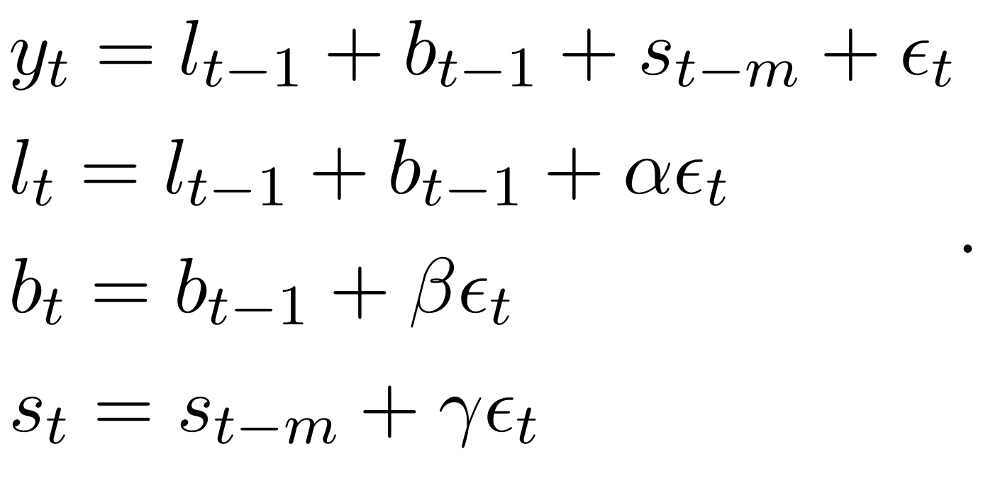
It is outdated and shows that you have completely ignored all the developments in the area since 1985 (side note: when reviewing papers, if I see that authors use this formulation, I automatically flag the paper as a major revision). You should use the modern approach instead, State Space Single Source of Error model, i.e. this formulation: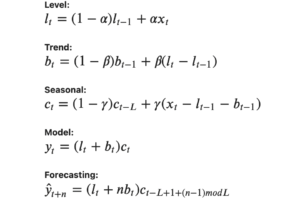
Outdated formulation of exponential smoothing
\begin{equation*}
\begin{aligned}
& {y}_{t} = l_{t-1} + b_{t-1} + s_{t-m} + \epsilon_t \\
& l_t = l_{t-1} + b_{t-1} + \alpha \epsilon_t \\
& b_t = b_{t-1} + \beta \epsilon_t \\
& s_t = s_{t-m} + \gamma \epsilon_t
\end{aligned} .
\end{equation*}If you see someone using the old formulation, know that they do not know the state-of-the-art forecasting.

Here are the slides of the presentation.
And here is the recording of the webinar: