Authors: Ivan Svetunkov, John E. Boylan

Journal: International Journal of Production Economics

Abstract: Inventory decisions relating to items that are demanded intermittently are particularly challenging. Decisions relating to termination of sales of product often rely on point estimates of the mean demand, whereas replenishment decisions depend on quantiles from interval estimates. It is in this context that modelling intermittent demand becomes an important task. In previous research, this has been addressed by generalised linear models or integer-valued ARMA models, while the development of models in state space framework has had mixed success. In this paper, we propose a general state space model that takes intermittence of data into account, extending the taxonomy of single source of error state space models. We show that this model has a connection with conventional non-intermittent state space models used in inventory planning. Certain forms of it may be estimated by Croston’s and Teunter-Syntetos-Babai (TSB) forecasting methods. We discuss properties of the proposed models and show how a selection can be made between them in the proposed framework. We then conduct a simulation experiment, empirically evaluating the inventory implications.

DOI: 10.1016/j.ijpe.2023.109013.

Working paper.

About the paper

DISCLAIMER: The models in this paper are also discussed in detail in the ADAM monograph (Chapter 13) with some examples going beyond what is discussed in the paper (e.g. models with trends).

What is “intermittent demand”? It is the demand that happens at irregular frequency (i.e. at random). Note that according to this definition, intermittent demand does not need to be count – it is a wider term than that. For example, electricity demand can be intermittent, but it is definitely not count. The definition above means that we do not necessarily know when specifically we will sell our product. From the modelling point of view, it means that we need to take into account two elements of uncertainty instead of just one:

1. How much people will buy;
2. When they will buy.

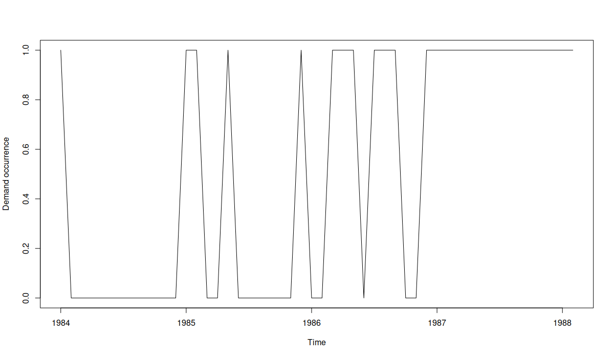
(1) is familiar for many demand planners and data scientists: we do not know specifically how much our customers will buy in the future, but we can get an estimate of the expected demand (mean value via a point forecast) and an idea of the uncertainty around it (e.g. produce prediction intervals or estimate the demand distribution). (2) is less obvious: there may be some periods when nobody buys our product, and then periods when we sell some, followed by no sales again. In that case we can encode the no sales in those “dry” periods with zeroes, the periods with demand as ones, and end up with a time series like this (this idea was briefly discussed in this and this posts):

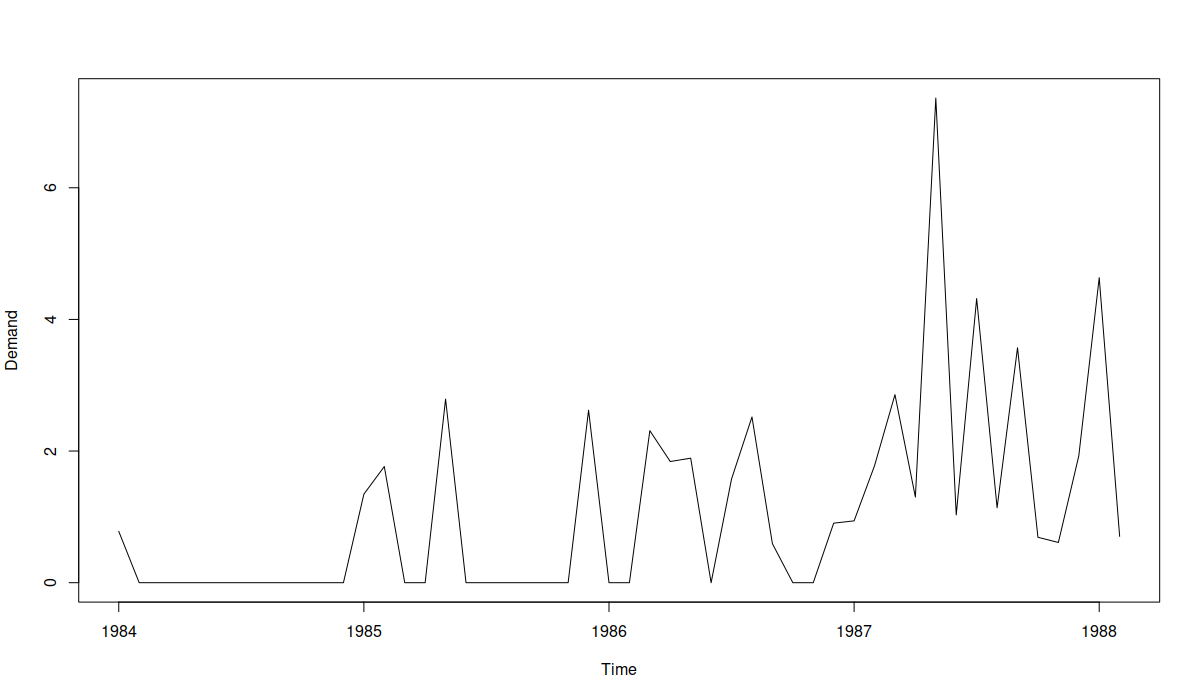
The plot above visualises the demand occurrence, with zeroes corresponding to the situation of “no demand” and ones corresponding to some demand. In general, it is is challenging to predict, when the “ones” will happen specifically, but in the case above, it seems that over time the frequency of demand increases, implying that maybe it becomes regular. In mathematical terms, we could phrase this as the probability of occurrence increases over time: at the end of series, we won’t necessarily sell product, but the chance of selling is much higher than in the beginning. The original time series looks like this:

It shows that indeed there is an increase of the frequency of sales together with the amount sold, and that it seems that the product is becoming more popular, moving from the intermittent to the regular demand domain.

In general, forecasting intermittent demand is a challenging task, but there are many existing approaches that can be used in this case. However, they are all detached from the conventional ones that are used for regular demand (such as ETS or ARIMA). What people usually do in practice is first categorise the data into regular and intermittent and then apply specific approaches to it (e.g. ETS/ARIMA for the regular demand, and Croston‘s method or TSB for the intermittent one).

John Boylan and I developed a statistical model that unites the two worlds – you no longer need to decide whether the data is intermittent or not, you can just use one model in an automated fashion – it will take care of intermittence (if there is one). It relies fundamentally on the classical Croston’s equation:
\begin{equation} \label{eq:general}
y_t = o_t z_t ,
\end{equation}
where \(y_t\) is the observed value at time \(t\), \(o_t\) is the binary occurrence variable and \(z_t\) is the demand sizes variable. Trying to derive the statistical model underlying Croston’s method, Snyder (2002) and Shenstone & Hyndman (2005) used models based on \eqref{eq:general} but instead of plugging in a multiplicative ETS in \(z_t\) they got stuck with the idea of logarithmic transformation of demand sizes and/or using count distributions for the demand sizes. John and I looked into this equation again and decided that we can model both demand sizes and demand occurrence using a pair of pure multiplicative ETS models. In this post, I will focus on ETS(M,N,N) as the simplest model, but more complicated ones (with trend and/or explanatory variables) can be used as well without the loss in logic. So, for the demand sizes we will have:
\begin{equation}
\begin{aligned}
& z_t = l_{t-1} (1 + \epsilon_t) \\
& l_t = l_{t-1} (1 + \alpha \epsilon_t)
\end{aligned}
\label{eq:demandSizes}
\end{equation}
where \(l_t\) is the level of series, \(\alpha\) is the smoothing parameter and \(1 + \epsilon_t \) is the error term that follows some positive distribution (the options we considered in the paper are the Log-Normal, Gamma and Inverse Gaussian). The demand sizes part is relatively straightforward: you just apply the conventional pure multiplicative ETS model with a positive distribution (which makes \(z_t\) always positive) and that’s it. However, the occurrence part is more complicated.

Given that the occurrence variable is random, we should model the probability of occurrence. We proposed to assume that \(o_t \sim \mathrm{Bernoulli}(p_t) \) (logical assumption, done in many other papers), meaning that the probability of occurrence changes over time. In turn, the changing probability can be modelled using one of the several approaches that we proposed. For example, it can be modelled via the so called “inverse odds ratio” model with ETS(M,N,N), formulated as:
\begin{equation}
\begin{aligned}
& p_t = \frac{1}{1 + \mu_{b,t}} \\
& \mu_{b,t} = l_{b,t-1} \\
& l_{b,t} = l_{b,t-1} (1 + \alpha_b \epsilon_{b,t})
\end{aligned}
\label{eq:demandOccurrenceOdds}
\end{equation}
where \(\mu_{b,t}\) is the one step ahead expectation of the underlying model, \(l_{b,t}\) is the latent level, \(\alpha_b\) is the smoothing parameter of the model, and \(1+\epsilon_{b,t}\) is the positively distributed error term (with expectation equal to one and an unknown distribution, which we actually do not care about). The main feature of the inverse odds ratio occurrence model is that it should be effective in cases when demand is building up (moving from the intermittent to the regular pattern, without zeroes). In our paper we show how such model can be estimated and also show that Croston’s method can be used for the estimation of this model when the demand occurrence does not change (substantially) between the non-zero demands. So, this model can be considered as the model underlying Croston’s method.

Uniting the equations \eqref{eq:general}, \eqref{eq:demandSizes} and \eqref{eq:demandOccurrenceOdds}, we get the iETS(M,N,N)\(_\mathrm{I}\)(M,N,N) model, where the letters in the first brackets correspond to the demand sizes part, the subscript “I” tells us that we have the “inverse odds ratio” model for the occurrence, and the second brackets show what ETS model was used in the demand occurrence model. The paper explains in detail how this model can be built and estimated.

In the very same paper we discuss other potential models for demand occurrence (more suitable for demand obsolescence or fixed probability of occurrence) and, in fact, in my opinion this part is the main contribution of the paper – we have looked into something no one did before: how to model demand occurrence using ETS. Having so many options, we might need to decide which to use in an automated fashion. Luckily, given that these models are formulated in one and the same framework, we can use information criteria to select the most suitable one for the data. Furthermore, when all probabilities of occurrence are equal to one, the model \eqref{eq:general} together with \eqref{eq:demandSizes} transforms into the conventional ETS(M,N,N) model. This also means that the regular ETS model can be compared with the iETS directly using information criteria to decide whether the occurrence part is needed or not. So, we end up with a relatively simple framework that can be used for any type of demand without a need to do a categorisation.

As a small side note, we also showed in the paper that the estimates of smoothing parameters for the demand sizes in iETS will always be positively biased (being higher than needed). In fact, this bias appears in any intermittent demand model that assumes that the potential demand sizes change between the non-zero observations (reasonable assumption for any modelling approach). In a way, this finding also applies to both Croston’s and TSB methods and agrees with similar finding by Kourentzes (2014).

Example in R

All the models from the paper are implemented in the adam() function from the smooth package in R (with the oes() function taking care of the occurrence, see details here and here). For the demonstration purposes (and for fun), we will consider an artificial example of the demand obsolescence, modelled via the “Direct probability” iETS model (it underlies the TSB method):

set.seed(7)
c(rpois(10,3),rpois(10,2),rpois(10,1),rpois(10,0.5),rpois(10,0.1)) |>
    ts(frequency=12) -> y

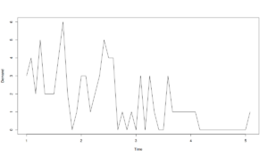
My randomly generated time series looks like this:

In practice, in the example above, we can be interested in deciding, whether to discontinue the product (to save money on stocking it) or not. To model and forecast the demand above, we can use the following code in R:

library(smooth)
iETSModel <- adam(y, "YYN", occurrence="direct", h=5, holdout=TRUE)

The "YYN" above tells function to select the best pure multiplicative ETS model based on the information criterion (AICc by default, see discussion in Section 15.1 of the ADAM monograph), the "occurrence" variable specifies, which of the demand occurrence models to build. By default, the function will use the same model for the demand probability as the selected for the demand sizes. So, for example, if we end up with ETS(M,M,N) for demand sizes, the function will use ETS(M,M,N) for the probability of occurrence. If you want to change this, you would need to use the oes() function and specify the model there (see examples in Section 13.4 of the ADAM monograph). Finally, I've asked function to produce 5 steps ahead forecasts and to keep the last 5 observations in the holdout sample. I ended up having the following model:

summary(iETSModel)

Model estimated using adam() function: iETS(MMN)
Response variable: y
Occurrence model type: Direct
Distribution used in the estimation: 
Mixture of Bernoulli and Gamma
Loss function type: likelihood; Loss function value: 71.0549
Coefficients:
      Estimate Std. Error Lower 2.5% Upper 97.5%  
alpha   0.1049     0.0925     0.0000      0.2903  
beta    0.1049     0.0139     0.0767      0.1049 *
level   4.3722     1.1801     1.9789      6.7381 *
trend   0.9517     0.0582     0.8336      1.0685 *

Error standard deviation: 1.0548
Sample size: 45
Number of estimated parameters: 9
Number of degrees of freedom: 36
Information criteria:
     AIC     AICc      BIC     BICc 
202.6527 204.1911 218.9126 206.6142 

As we see from the output above, the function has selected the iETS(M,M,N) model for the data. The line "Mixture of Bernoulli and Gamma" tells us that the Bernoulli distribution was used for the demand occurrence (this is the only option), while the Gamma distribution was used for the demand sizes (this is the default option, but you can change this via the distribution parameter). We can then produce forecasts from this model:

forecast(iETSModel, h=5, interval="prediction", side="upper") |>
    plot()

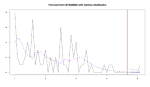
In the code above, I have asked the function to generate prediction intervals (by default, for the pure multiplicative models, the function uses simulations) and to produce only the upper bound of the interval. The latter is motivated by the idea that in the case of the intermittent demand, the lower bound is typically not useful for decision making: we know that the demand cannot be below zero, and our stocking decisions are typically made based on the specific quantiles (e.g. for the 95% confidence level). Here is the plot that I get after running the code above:

While the last observation in the holdout was not included in the prediction interval, the dynamics captured by the model is correct. The question that we should ask ourselves in this example is: what decision can be made based on the model? If you want to decide whether to stock the product or not, you can look at the forecast of the probability of occurrence to see how it changes over time and decide, whether to discontinue the product:

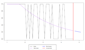
forecast(iETSModel$occurrence, h=5) |> plot()

In our case, the probability reaches roughly 0.2 over the next 5 months (i.e. we might sale once every 5 months). If we think that this is too low then we should discontinue the product. Otherwise, if we decide to continue selling the product, then it makes more sense to generate the desired quantile of the cumulative demand over the lead time. In case of the adam() function it can be done by adding cumulative=TRUE in the forecast() function:

forecast(iETSModel, h=5, interval="prediction", side="upper", cumulative=TRUE)

after which we get:

      Point forecast Upper bound (95%)
Oct 4      0.3055742          1.208207

From the decision point of view, if we deal with count demand, the value 1.208207 complicates things. Luckily, as we showed in our paper, we can round the value up to get something meaningful, preserving the properties of the model. This means, that based on the estimated model, we need to have two items in stock to satisfy the demand over the next 5 months with the confidence level of 95%.

Conclusions

This is just a demonstration of what can be done with the proposed iETS model, but there are many more things one can do. For example, this approach allows capturing multiplicative seasonality in data that has zeroes (as long as seasonal indices can be estimated somehow). John and I started thinking in this direction, and we even did some work together with Patricia Ramos (our colleague from the university of INESC TEC), but given the hard time that was given to our paper by the reviewers in IJF, we had to postpone this research. I also used the ideas explained in this post in the paper on ED forecasting (written together with Bahman and Jethro). In that paper, I have used a seasonal model with the "direct" occurrence part, which tool care of zeroes (not bothering with modelling them properly) and allowed me to apply a multiple seasonal multiplicative ETS model with explanatory variables. Anyway, the proposed approach is flexible enough to be used in variety of contexts, and I think it will have many applications in real life.

P.S.: Story of the paper

I've written a separate long post, explaining the revision process of the paper and how it got to the acceptance stage at the IJPE, but then I realised that it is too long and boring. Besides, John would not have approved of the post and would say that I am sharing the unnecessary details, creating potential exasperation for fellow forecasters who reviewed the paper. So, I have decided not to publish that post, and instead just to add a short subsection. Here it is.

We started working on the paper in March 2016 and submitted it to the International Journal of Forecasting (IJF) in January 2017. It went through four rounds of revision with the second reviewer throughout the way being very critical, unsupportive and driving the paper into a wrong direction, burying it in the discussion of petty statistical details. We rewrote the paper several times and I rewrote the R code of the function few times. In the end the Associate Editor (AE) of the IJF (who completely forgot about our paper for several months) decided not to send the paper to the reviewers again, completely ignored our responses to the reviewers, did not provide any major feedback and have written an insulting response that ended with the phrase "I could go on, but I’m out of patience with the authors and their paper". The paper was rejected from IJF in 2019, which set me back in my academic career. This together with constant rejections of my Complex Exponential Smoothing paper and actions of a colleague of mine who decided to cut all ties with me in Summer 2019, hit my self-esteem and caused a serious damage to my professional life. I thought of quitting academia and to either starting working in business or doing something different with my life, not related to forecasting at all. I stayed mainly because of all the support that John Boylan, Robert Fildes, Nikos Kourentzes and my wife Anna Sroginis provided me. I recovered from that hit only in 2022, when my Complex Exponential Smoothing paper got accepted and things finally started turning well. After that John and I have rewritten the paper again, split it into two: "iETS" and "Multiplicative ETS" (under revision in IMA Journal of Management Mathematics) and submitted the former to the International Journal of Production Economics, where after one round of revision it got accepted. Unfortunately, we never got to celebrate the success with John because he passed away.

The moral of this story is that publishing in academia can be very tough and unfair. Sometimes, you get a very negative feedback from the people you least expect to get it from. People that you respect and think very highly of might not understand what you are proposing and be very unsupportive. We actually knew who the reviewers and the AE of our IJF paper were - they are esteemed academics in the field of forecasting. And while I still think highly of their research and contributions to the field, the way the second reviewer and the AE handled the review has damaged my personal respect to them - I never expected them to be so narrow-minded...