
ARIMA has been a workhorse for decades. But the standard implementations quietly hard-code assumptions: one seasonal cycle, Gaussian errors, regressors handled separately etc. This is fine for textbook well-behaved data. But what do you do when you face real data?
The conventional implementations (statsmodels or pmdarima in Python, stats in R) do their job well: they estimate SARIMA via likelihood, select orders automatically, and produce sensible forecasts for series with trend and one seasonality. Monthly or quarterly demand data is their home ground. The problems start when the data has more than one cycle: the classical SARIMA formulation has a slot for exactly one seasonal lag, so for the half-hourly electricity demand you would have to pick either the hour-of-day or the day-of-week cycle and discard the other.
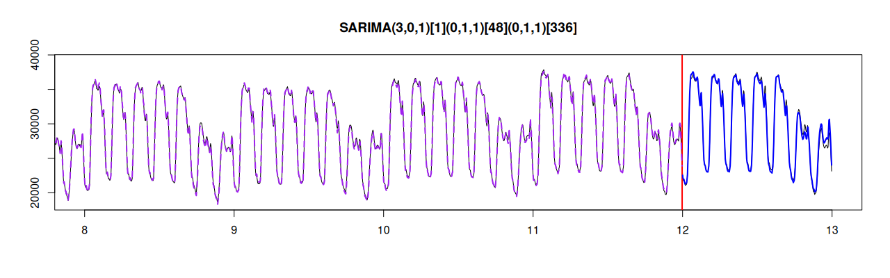
MSARIMA (Multiple Seasonal ARIMA) solves this by reformulating ARIMA in the Single Source of Error (SSOE) state space form. Each AR, I, and MA element becomes a state in the model, so nothing restricts you to one seasonal lag: you can have as many as you want. In the smooth package, orders are specified per lag, matched to a lags list. Here is an example on the classical taylor series (half-hourly electricity demand in England and Wales), with two seasonal cycles:
from fcompdata import taylor

from smooth import MSARIMA
# MSARIMA(3,0,1)(0,1,1)[48](0,1,1)[336]
model = MSARIMA(
orders={"ar": [3, 0, 0], "i": [0, 1, 1], "ma": [1, 1, 1]},
lags=[1, 48, 336],
h=336, holdout=True
)
model.fit(taylor.y)
model.predict(h=336, interval="prediction", level=0.95)
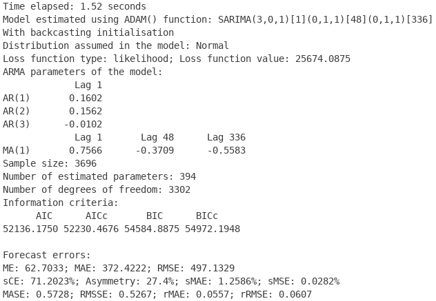
In Python, it takes only 1.5 seconds for the function to fit the model to the data and estimate its parameters, which is fast for a double-seasonal model fit to roughly four thousand observations:
But the smooth implementation brings several additional practical benefits.
First, model.fit() accepts a matrix of external regressors via xreg, estimated jointly with the ARIMA components – no separate pre-filtering step. The logic and the code are identical to ETSX, which I covered earlier.
Second, you can swap the loss: loss=”GTMSE” or “MSEh” optimises the model directly on multistep errors, with the same shrinkage mechanism I discussed in the post on multistep losses.
Third, you don’t need to stick with the Gaussian distribution – you can choose other ones if you think that, for example, Laplace is more suitable for the data (this post).
And there is one more thing. Because MSARIMA now lives in the same state space framework as ETS, the two models can be combined into one and compared with each other directly via information criteria. But that deserves a post of its own, so stay tuned.
Read Chapter 9 on ADAM ARIMA.
Or check out the documentation in smooth wiki.
An why not try it yourself? pip install smooth