After working on this for more than a year, I have finally prepared the first draft of my online monograph “Forecasting and Analytics with ADAM“. This is a monograph on the model that unites ETS, ARIMA and regression and introduces advanced features in univariate modelling, including:

1. ETS in a new State Space form;
2. ARIMA in a new State Space form;
3. Regression;
4. TVP regression;
5. Combinations of (1), (2) and either (3), or (4);
6. Automatic selection/combination for ETS;
7. Automatic orders selection for ARIMA;
8. Variables selection for regression part;
9. Normal and non-normal distributions;
10. Automatic selection of most suitable distribution;
11. Multiple seasonality;
12. Occurrence part of the model to handle zeroes in data (intermittent demand);
13. Modelling scale of distribution (GARCH and beyond);
14. Handling uncertainty of estimates of parameters.

The model and all its features are already implemented in adam() function from smooth package for R (you need v3.1.6 from CRAN for all the features listed above). The function supports many options that allow one experimenting with univariate forecasting, allowing to build complex models, combining elements from the list above. The monograph explaining how models underlying ADAM and how to work with them is available online, and I plan to produce several physical copies of it after refining the text. Furthermore, I have already asked two well-known academics to act as reviewers of the monograph to collect the feedback and improve the monograph, and if you want to act as a reviewer as well, please let me know.

Examples in R

Just to give you a flavour of ADAM, I decided to provide a couple of examples on time series AirPassengers (included in datasets package in R). The first one is the ADAM ETS.

Building and selecting the most appropriate ADAM ETS comes to running the following line of code:

adamETSAir <- adam(AirPassengers, h=12, holdout=TRUE)

In this case, ADAM will select the most appropriate ETS model for the data, creating a holdout of the last 12 observations. We can see the details of the model by printing the output:

adamETSAir

Time elapsed: 0.75 seconds
Model estimated using adam() function: ETS(MAM)
Distribution assumed in the model: Gamma
Loss function type: likelihood; Loss function value: 467.2981
Persistence vector g:
 alpha   beta  gamma 
0.7691 0.0053 0.0000 

Sample size: 132
Number of estimated parameters: 17
Number of degrees of freedom: 115
Information criteria:
      AIC      AICc       BIC      BICc 
 968.5961  973.9646 1017.6038 1030.7102 

Forecast errors:
ME: 9.537; MAE: 20.784; RMSE: 26.106
sCE: 43.598%; Asymmetry: 64.8%; sMAE: 7.918%; sMSE: 0.989%
MASE: 0.863; RMSSE: 0.833; rMAE: 0.273; rRMSE: 0.254

The output above provides plenty of detail on what was estimated and how. Some of these elements have been discussed in one of my previous posts on es() function. The new thing is the information about the assumed distribution for the response variable. By default, ADAM works with Gamma distribution in case of multiplicative error model. This is done to make model more robust in cases of low volume data, where the Normal distribution might produce negative numbers (see my presentation on this issues). In case of high volume data, the Gamma distribution will perform similar to the Normal one. The pure multiplicative ADAM ETS is discussed in Chapter 6 of ADAM monograph. If Gamma is not suitable, then the other distribution can be selected via the distribution parameter. There is also an automated distribution selection approach in the function auto.adam():

adamETSAutoAir <- auto.adam(AirPassengers, h=12, holdout=TRUE)
adamETSAutoAir

Time elapsed: 3.86 seconds
Model estimated using auto.adam() function: ETS(MAM)
Distribution assumed in the model: Normal
Loss function type: likelihood; Loss function value: 466.0744
Persistence vector g:
 alpha   beta  gamma 
0.8054 0.0000 0.0000 

Sample size: 132
Number of estimated parameters: 17
Number of degrees of freedom: 115
Information criteria:
      AIC      AICc       BIC      BICc 
 966.1487  971.5172 1015.1564 1028.2628 

Forecast errors:
ME: 9.922; MAE: 21.128; RMSE: 26.246
sCE: 45.36%; Asymmetry: 65.4%; sMAE: 8.049%; sMSE: 1%
MASE: 0.877; RMSSE: 0.838; rMAE: 0.278; rRMSE: 0.255

As we see from the output above, the Normal distribution is more appropriate for the data in terms of AICc than the other ones tried out by the function (by default the list includes Normal, Laplace, S, Generalised Normal, Gamma, Inverse Gaussian and Log Normal distributions, but this can be amended by providing a vector of names via distribution parameter). The selection of ADAM ETS and distributions is discussed in Chapter 15 of the monograph.

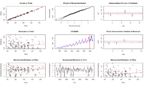
Having obtained the model, we can diagnose it using plot.adam() function:

par(mfcol=c(3,3))
plot(adamETSAutoAir,which=c(1,4,2,6,7,8,10,11,13))

The which parameter specifies what type of plots to produce, you can find the list of plots in the documentation for plot.adam(). The code above will result in:

The diagnostic plots are discussed in the Chapter 14 of ADAM monograph. The plot above does not show any serious issues with the model.

Just for the comparison, we could also try fitting the most appropriate ADAM ARIMA to the data (this model is discussed in Chapter 9). The code in this case is slightly more complicated, because we need to switch off ETS part of the model and define the maximum orders of ARIMA to try:

adamARIMAAir <- adam(AirPassengers, model="NNN", h=12, holdout=TRUE,
                     orders=list(ar=c(3,2),i=c(2,1),ma=c(3,2),select=TRUE))

This results in the following automatically selected ARIMA model:

Time elapsed: 3.54 seconds
Model estimated using auto.adam() function: SARIMA(0,1,1)[1](0,1,1)[12]
Distribution assumed in the model: Normal
Loss function type: likelihood; Loss function value: 491.7117
ARMA parameters of the model:
MA:
 theta1[1] theta1[12] 
   -0.1952    -0.0720 

Sample size: 132
Number of estimated parameters: 16
Number of degrees of freedom: 116
Information criteria:
     AIC     AICc      BIC     BICc 
1015.423 1020.154 1061.548 1073.097 

Forecast errors:
ME: -13.795; MAE: 16.65; RMSE: 21.644
sCE: -63.064%; Asymmetry: -79.4%; sMAE: 6.343%; sMSE: 0.68%
MASE: 0.691; RMSSE: 0.691; rMAE: 0.219; rRMSE: 0.21

Given that ADAM ETS and ADAM ARIMA are formulated in the same framework, they are directly comparable using information critirea. Comparing AICc of the models adamETSAutoAir and adamARIMAAir, we can conclude that the former is more appropriate to the data than the latter. However, the default ARIMA works with the Normal distribution, which might not be appropriate for the data, so we can revert to the auto.adam() to select the better one:

adamAutoARIMAAir <- auto.adam(AirPassengers, model="NNN", h=12, holdout=TRUE,
                              orders=list(ar=c(3,2),i=c(2,1),ma=c(3,2),select=TRUE))

This will take more computational time, but will result in a different model with a lower AICc (which is still higher than the one in ADAM ETS):

Time elapsed: 25.46 seconds
Model estimated using auto.adam() function: SARIMA(0,1,1)[1](0,1,1)[12]
Distribution assumed in the model: Log-Normal
Loss function type: likelihood; Loss function value: 472.923
ARMA parameters of the model:
MA:
 theta1[1] theta1[12] 
   -0.2785    -0.5530 

Sample size: 132
Number of estimated parameters: 16
Number of degrees of freedom: 116
Information criteria:
      AIC      AICc       BIC      BICc 
 977.8460  982.5764 1023.9708 1035.5197 

Forecast errors:
ME: -12.968; MAE: 13.971; RMSE: 19.143
sCE: -59.285%; Asymmetry: -91.7%; sMAE: 5.322%; sMSE: 0.532%
MASE: 0.58; RMSSE: 0.611; rMAE: 0.184; rRMSE: 0.186

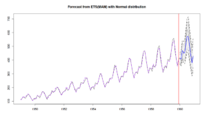
Note that although the AICc is higher for ARIMA than for ETS, the former has lower error measures than the latter. So, the higher AICc does not necessarily mean that the model is not good. But if we rely on the information criteria, then we should stick with ADAM ETS and we can then produce the forecasts for the next 12 observations (see Chapter 18):

adamETSAutoAirForecast <- forecast(adamETSAutoAir, h=12, interval="prediction",
                                   level=c(0.9,0.95,0.99))
par(mfcol=c(1,1))
plot(adamETSAutoAirForecast)

Finally, if we want to do a more in-depth analysis of parameters of ADAM, we can also produce the summary, which will create the confidence intervals for the parameters of the model:

summary(adamETSAutoAir)

Model estimated using auto.adam() function: ETS(MAM)
Response variable: data
Distribution used in the estimation: Normal
Loss function type: likelihood; Loss function value: 466.0744
Coefficients:
            Estimate Std. Error Lower 2.5% Upper 97.5%  
alpha         0.8054     0.0864     0.6343      0.9761 *
beta          0.0000     0.0203     0.0000      0.0401  
gamma         0.0000     0.0382     0.0000      0.0755  
level        96.2372     6.8596    82.6496    109.7919 *
trend         2.0901     0.3955     1.3068      2.8716 *
seasonal_1    0.9145     0.0077     0.9003      0.9372 *
seasonal_2    0.8999     0.0081     0.8857      0.9227 *
seasonal_3    1.0308     0.0094     1.0165      1.0535 *
seasonal_4    0.9885     0.0077     0.9743      1.0112 *
seasonal_5    0.9856     0.0072     0.9713      1.0083 *
seasonal_6    1.1165     0.0093     1.1023      1.1392 *
seasonal_7    1.2340     0.0115     1.2198      1.2568 *
seasonal_8    1.2254     0.0105     1.2112      1.2481 *
seasonal_9    1.0668     0.0094     1.0526      1.0896 *
seasonal_10   0.9256     0.0087     0.9113      0.9483 *
seasonal_11   0.8040     0.0075     0.7898      0.8268 *

Error standard deviation: 0.0367
Sample size: 132
Number of estimated parameters: 17
Number of degrees of freedom: 115
Information criteria:
      AIC      AICc       BIC      BICc 
 966.1487  971.5172 1015.1564 1028.2628 

Note that the summary() function might complain about the Observed Fisher Information. This is because the covariance matrix of parameters is calculated numerically and sometimes the likelihood is not maximised properly. I have not been able to fully resolve this issue yet, but hopefully will do at some point. The summary above shows, for example, that the smoothing parameters \(\beta\) and \(\gamma\) are not significantly different from zero (on 5% level), while \(\alpha\) is expected to vary between 0.6343 and 0.9761 in 95% of the cases. You can read more about the uncertainty of parameters in ADAM in Chapter 16 of the monograph.

As for the other features of ADAM, here is a brief guide:

• If you work with multiple seasonal data, then you might need to specify the seasonality via the lags parameter, for example as lags=c(24,7*24) in case of hourly data. This is discussed in Chapter 12;
• If you have intermittent data, then you should read Chapter 13, which explains how to work with the occurrence parameter of the function;
• Explanatory variables are discussed in Chapter 10 and are handled in the adam() function via the formula parameter;
• In the cases of heteroscedasticity (time varying or induced by some explanatory variables), there a scale model (which is discussed in Chapter 17 and implemented as sm() method for the adam class).

You can also experiment with advanced estimators (Chapter 11, including custom loss functions) via the loss parameter and forecast combinations (Section 15.4).

Long story short, if you are interested in univariate forecasting, then do give ADAM a try - it might have the flexibility you needed for your experiments. If you are worried about its accuracy, check out this post, where I compared ADAM with other models.

And, as a friend of mine says, "Happy forecasting!"