
Have you ever tried to identify ARIMA for your data? The old school Box-Jenkins methodology implies analysing ACF/PACF plots and selecting the orders iteratively. This approach has a fundamental flaw I discussed in one of my earlier posts. Brute force does not help either: even p ≤ 3, d ≤ 2, q ≤ 3 gives 48 candidates, and seasonal lags push it into the thousands. So, smart people came up with great heuristics that allow identifying the orders in a short period of time. Let me explain.
One of the widely used approaches was developed by Hyndman & Khandakar (2008). It is implemented in auto.arima in R (and in StatsForecast for Python). It mixes two frameworks: stationarity tests (KPSS or ADF) to select the order of differencing d, and then information criteria for p and q. The tests are needed because, in the conventional formulation, models with different d are estimated on different sample sizes, so their information criteria cannot be compared (I explained this here). Although the algorithm works well and showed good performance in several competitions, it mixes hypothesis testing with information theory. The former tests the differences between samples, but assumes that you can make a mistake (based on your significance level), while the latter simply selects the most plausible model given data.
AutoMSARIMA does the selection differently. Because it is formulated in state space, the sample stays the same for any d, so the algorithm can compare all orders directly via information criteria, including the differencing. This follows the approach of Svetunkov & Boylan (2020), which treats order selection as a component selection problem rather than hypothesis testing. No ADF test, no KPSS test, no pre-screening for stationarity. The IC decides everything. And because nothing in this logic is tied to a specific seasonal period, it extends naturally to multiple seasonalities: each seasonal lag simply adds its own components to the model, and the same criterion decides which of them to keep, with the seasonality remaining stochastic rather than fixed.
The search itself is stepwise: the algorithm inspects the ACF/PACF of the residuals to propose a candidate order, adds it, and keeps it only if the information criterion decreases. When done, it also tries several simple SARIMA models to check whether any of them beats the selected one. The algorithm is explained in detail here.
In Python:
from fcompdata import AirPassengers
from smooth import AutoMSARIMA

# Monthly data, automatic order selection up to SARIMA(3,2,3)(3,1,3)[12]
model = AutoMSARIMA(lags=[1, 12])
model.fit(AirPassengers.y)
print(model)
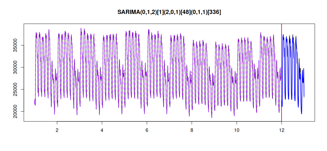
The same algorithm works for the multiple seasonal ARIMA. The only thing to specify explicitly is the maximum orders to check:
from fcompdata import taylor

model = AutoMSARIMA(
lags=[1, 48, 336],
orders={"ar": [3, 2, 2],
"i": [2, 1, 1],
"ma": [3, 2, 2]}
)
model.fit(taylor.y)
The selected model returns the same attributes and supports the same methods as ADAM.
Does it actually work? I benchmarked AutoMSARIMA against statsforecast AutoARIMA, skforecast and R’s auto.arima on 5,315 series from the M1, M3 and Tourism datasets. The honest summary: point accuracy is a tie – RMSSE differs in the third decimal place across all implementations. But smooth produces the best-calibrated prediction intervals of the pack and is 3–5 times faster than the alternatives. Here is the full notebook.
Try smooth now: pip install smooth
smooth wiki.