


Back in 2020, when we were all siting in the COVID lockdown, I had a call with Bahman Rostami-Tabar to discuss one of our projects. He told me that he had an hourly data of an Emergency Department from a hospital in Wales, and suggested writing a paper for a healthcare audience to show them how forecasting can be done properly in this setting. I noted that we did not have experience in working with high frequency data, and it would be good to have someone with relevant expertise. I knew a guy who worked in energy forecasting, Jethro Browell (we are mates in the IIF UK Chapter), so we had a chat between the three of us and formed a team to figure out better ways for ED arrival demand forecasting.
We agreed that each one of us will try their own models. Bahman wanted to try TBATS, Prophet and models from the fasster package in R (spoiler: the latter ones produced very poor forecasts on our data, so we removed them from the paper). Jethro had a pool of GAMLSS models with different distributions, including Poisson and truncated Normal. He also tried a Gradient Boosting Machine (GBM). I decided to test ETS, Poisson Regression and ADAM. We agreed that we will measure performance of models not only in terms of point forecasts (using RMSE), but also in terms of quantiles (pinball and quantile bias) and computational time. It took us a year to do all the experiments and another one to find a journal that would not desk-reject our paper because the editor thought that it was not relevant (even though they have published similar papers in the past). It was rejected from Annals of Emergency Medicine, Emergency Medicine Journal, American Journal of Emergency Medicine and Journal of Medical Systems. In the end, we submitted to Health Systems, and after a short revision the paper got accepted. So, there is a happy end in this story.
In the paper itself, we found that overall, in terms of quantile bias (calibration of models), GAMLSS with truncated Normal distribution and ADAM performed better than the other approaches, with the former also doing well in terms of pinball loss and the latter doing well in terms of point forecasts (RMSE). Note that the count data models did worse than the continuous ones, although one would expect Poisson distribution to be appropriate for the ED arrivals.
I don’t want to explain the paper and its findings in detail in this post, but given my relation to ADAM, I have decided to briefly explain what I included in the model and how it was used. After all, this is the first paper that uses almost all the main features of ADAM and shows how powerful it can be if used correctly.
Using ADAM in Emergency Department arrivals forecasting
Disclaimer: The explanation provided here relies on the content of my monograph “Forecasting and Analytics with ADAM“. In the paper, I ended up creating a quite complicated model that allowed capturing complex demand dynamics. In order to fully understand what I am discussing in this post, you might need to refer to the monograph.
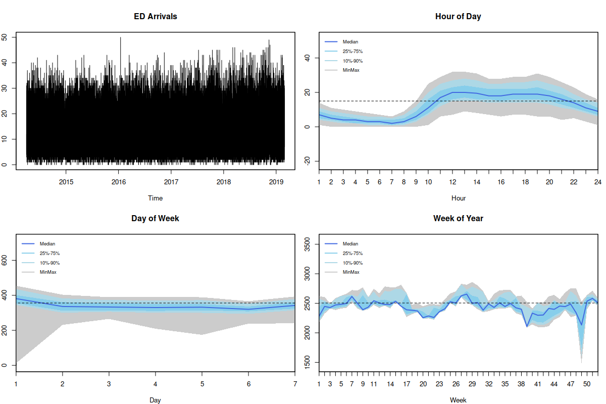
Emergency Department Arrivals. The plots were generated using seasplot() function from the tsutils package.
The figure above shows the data that we were dealing with together with several seasonal plots (generated using seasplot() function from the tsutils package). As we see, the data exhibits hour of day, day of week and week of year seasonalities, although some of them are not very well pronounced. The data does not seem to have a strong trend, although there is a slow increase of the level. Based on this, I decided to use ETS(M,N,M) as the basis for modelling. However, if we want to capture all three seasonal patterns then we need to fit a triple seasonal model, which requires too much computational time, because of the estimation of all the seasonal indices. So, I have decided to use a double-seasonal ETS(M,N,M) instead with hour of day and hour of week seasonalities and to include dummy variables for week of year seasonality. The alternative to week of year dummies would be hour of year seasonal component, which would then require estimating 8760 seasonal indices, potentially overfitting the data. I argue that the week of year dummy provides the sufficient flexibility and there is no need in capturing the detailed intra-yearly profile on a more granular level.
To make things more exciting, given that we deal with hourly data of a UK hospital, we had to deal with issues of daylight saving and leap year. I know that many of us hate the idea of daylight saving, because we have to change our lifestyles 2 times each year just because of an old 18th century tradition. But in addition to being bad for your health, this nasty thing messes things up for my models, because once a year we have 23 hours and in another time we have 25 hours in a day. Luckily, it is taken care of by adam() that shifts seasonal indices, when the time change happens. All you need to do for this mechanism to work is to provide an object with timestamps to the function (for example, zoo). As for the leap year, it becomes less important when we model week of year seasonality instead of the day of year or hour of year one.
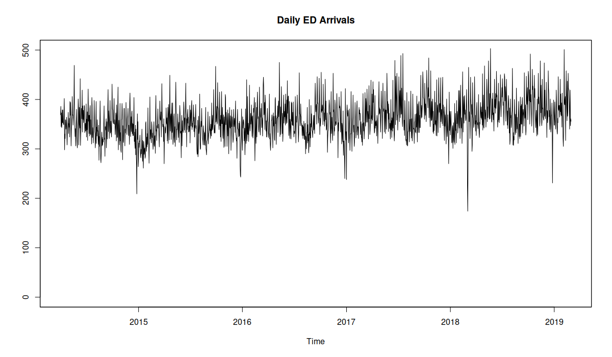
Emergency Department Daily Arrivals
Furthermore, as it can be seen from the figure above, it is apparent that calendar events play a crucial role in ED arrivals. For example, the Emergency Department demand over Christmas is typically lower than average (the drops in Figure above), but right after the Christmas it tends to go up (with all the people who injured themselves during the festivities showing up in the hospital). So these events need to be taken into account in a form of additional dummy variables by a model together with their lags (the 24 hour lags of the original variables).
But that’s not all. If we want to fit a multiplicative seasonal model (which makes more sense than the additive one due to changing seasonal amplitude for different times of year), we need to do something with zeroes, which happen naturally in ED arrivals over night (see the first figure in this post with seasonal plots). They do not necessarily happen at the same time of day, but the probability of having no demand tends to increase at night. This meant that I needed to introduce the occurrence part of the model to take care of zeroes. I used a very basic occurrence model called “direct probability“, because it is more sensitive to changes in demand occurrence, making the model more responsive. I did not use a seasonal demand occurrence model (and I don’t remember why), which is one of the limitations of ADAM used in this study.
Finally, given that we are dealing with low volume data, a positive distribution needed to be used instead of the Normal one. I used Gamma distribution because it is better behaved than the Log Normal or the Inverse Gaussian, which tend to have much heavier tails. In the exploration of the data, I found that Gamma does better than the other two, probably because the ED arrivals have relatively slim tails.
So, the final ADAM included the following features:
- ETS(M,N,M) as the basis;
- Double seasonality;
- Week of year dummy variables;
- Dummy variables for calendar events with their lags;
- “Direct probability” occurrence model;
- Gamma distribution for the residuals of the model.
This model is summarised in equation (3) of the paper.
The model was initialised using backcasting, because otherwise we would need to estimate too many initial values for the state vector. The estimation itself was done using likelihood. In R, this corresponded to roughly the following lines of code:
library(smooth)
oesModel <- oes(y, "MNN", occurrence="direct", h=48)
adamModelFirst <- adam(ourData, "MNM", lags=c(24,24*7), formula=y~x+xLag24+weekOfYear,
                       h=48, initial="backcasting",
                       occurrence=oesModel, distribution="dgamma")
Where x was the categorical variable (factor in R) with all the main calendar events. However, even with backcasting, the estimation of such a big model took an hour and 25 minutes. Given that Bahman, Jethro and I have agreed to do rolling origin evaluation, I've decided to help the function in the estimation inside the loop, providing the initials to the optimiser based on the very first estimated model. As a result, each estimation of ADAM in the rolling origin took 1.5 minutes. The code in the loop was modified to:
adamParameters <- coef(adamModelFirst)
oesModel <- oes(y, "MNN", occurrence="direct", h=48)
adamModel <- adam(ourData, "MNM", lags=c(24,24*7), formula=y~x+xLag24+weekOfYear,
                  h=48, initial="backcasting",
                  occurrence=oesModel, distribution="dgamma",
                  B=adamParameters)
Finally, we generated mean and quantile forecasts for 48 hours ahead. I used semiparametric quantiles, because I expected violation of some of assumptions in the model (e.g. autocorrelated residuals). The respective R code is:
testForecast <- forecast(adamModel, newdata=newdata, h=48,
                         interval="semiparametric", level=c(1:19/20), side="upper")
Furthermore, given that the data is integer-valued (how many people visit the hospital each hour) and ADAM produces fractional quantiles (because of the Gamma distribution), I decided to see how it would perform if the quantiles were rounded up. This strategy is simple and might be sensible when a continuous model is used for forecasting on a count data (see discussion in the paper). However, after running the experiment, the ADAM with rounded up quantiles performed very similar to the conventional one, so we have decided not to include it in the paper.
In the end, as stated earlier in this post, we concluded that in our experiment, there were two well performing approaches: GAMLSS with Truncated Normal distribution (called "NOtr-2" in the paper) and ADAM in the form explained above. The popular TBATS, Prophet and Gradient Boosting Machine performed poorly compared to these two approaches. For the first two, this is because of the lack of explanatory variables and inappropriate distributional assumptions (normality). As for the GBM, this is probably due to the lack of dynamic element in it (e.g. changing level and seasonal components).
Concluding this post, as you can see, I managed to fit a decent model based on ADAM, which captured the main characteristics of the data. However, it took a bit of time to understand what features should be included, together with some experiments on the data. This case study shows that if you want to get a better model for your problem, you might need to dive in the problem and spend some time analysing what you have on hands, experimenting with different parameters of a model. ADAM provides the flexibility necessary for such experiments.