
Have you heard of Croston’s method for intermittent demand forecasting? Some modern data scientists dislike it because it is too simple and not as accurate as some modern forecasting approaches. And they have a point. But here is why it is worth keeping Croston in mind.
Back in 1972, John Croston, who worked on stock control systems relying on Simple Exponential Smoothing (SES), noticed that SES forecasts were biased exactly when ordering decisions were made: right after a demand occurred. The following image shows why.
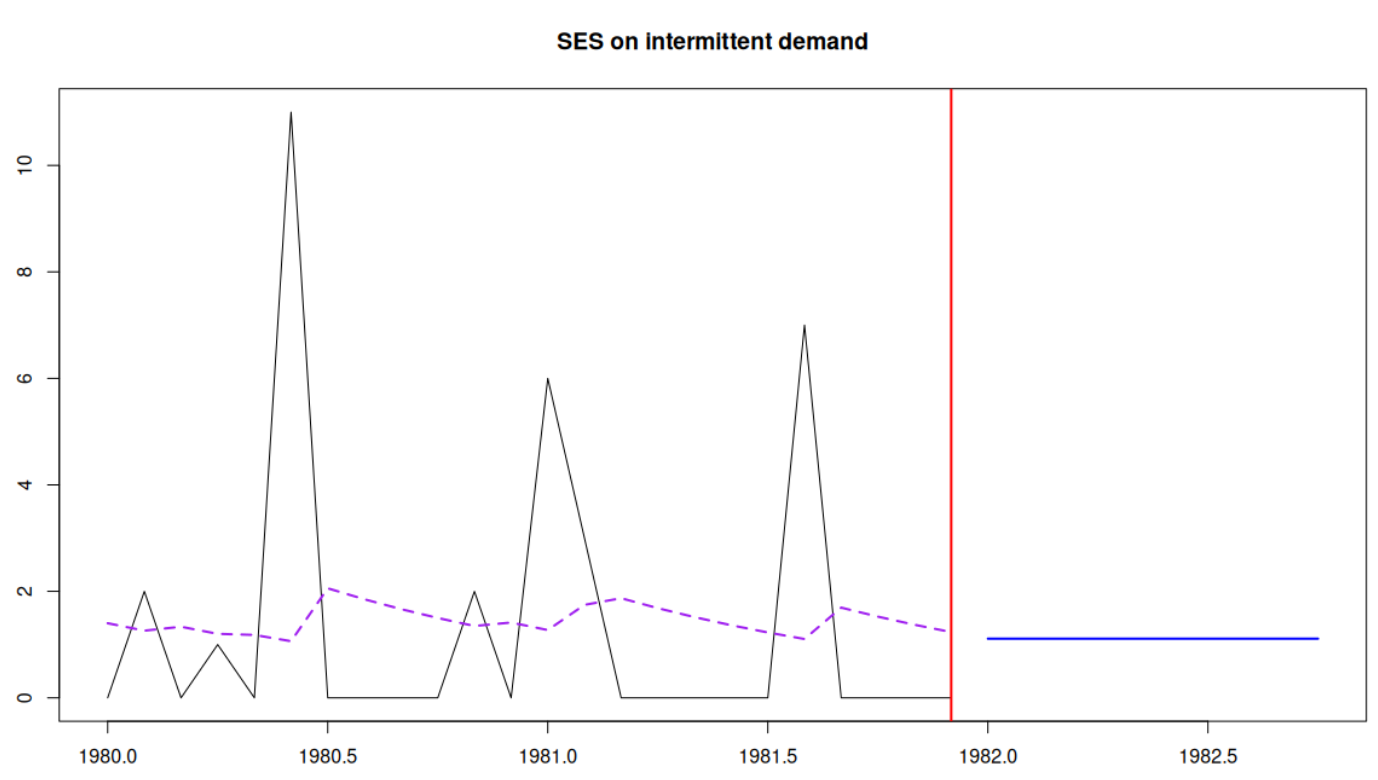
Intermittent demand consists mostly of periods with no sales, and SES treats each of them as a sale of size zero rather than as the absence of a sale. So, its forecast goes down with every zero, as if people wanted the product less and less. Then a customer buys 5 units, and SES immediately becomes optimistic. But in intermittent demand, sales rarely happen in consecutive periods, so this optimism leads to wrong ordering decisions.
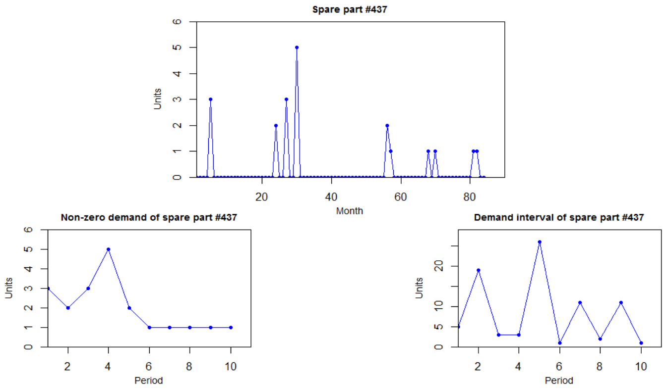
The problem is not SES itself, but that it does not distinguish demand occurrence from demand sizes. Croston split the series into two parts (see the main image of the post): demand intervals (the number of periods between non-zero demands) and demand sizes (the non-zero values). He applied SES to each of them separately, and defined the final forecast as the ratio of the smoothed sizes to the smoothed intervals, i.e. the expected demand per period. Both parts are updated only when a demand happens, so the method does not change its mind with every zero, giving more stable forecasts and more reasonable ordering decisions.
Nowadays, we have many great forecasting approaches, from simple ones like TSB to more advanced ones like LightGBM. Croston’s method itself turned out to be biased (Syntetos & Boylan proposed a correction for that). Still, it works fine for manufacturers of large expensive items, with low volumes and long gaps between orders, where a stable forecast matters more than a quick reaction. I am not a big fan of the method, but I really like Croston’s original idea: split intermittent demand into demand occurrence and demand sizes. More than half a century later, this idea still works. My iETS paper used it, outperforming other simple forecasting methods on the M5 data. Türkmen et al. (2021) used the same idea with deep neural networks. The paper with Anna Sroginis showed that it also works with LightGBM, leading to substantial accuracy improvements that translate into inventory savings. So, even if you dislike Croston’s method, I bet you can improve your approach by using his original idea.
We will cover intermittent demand and the methods built on Croston’s idea in our Demand Forecasting Principles course in November.