
In one of the comments to my previous post about the Simple Moving Average on LinkedIn, a reader mentioned that they use a Weighted Moving Average with their own weighting scheme. This can work well although defining the weights can be a nuisance: a Weighted Moving Average of order 12 needs 12 weights that someone has to choose. But what if one number could define them all?
First, why would we want non-equal weights in the first place? Demand evolves over time, and recent sales might reflect its current level better than the sales we had several years ago. So, it is only natural to give higher weights to recent observations and lower ones to older ones. Can we do that in a simple and principled way? Yes, and there is a forecasting method that does exactly that!
I’m talking about Simple Exponential Smoothing (SES), proposed by Robert Goodell Brown back in 1956 and independently by Charles Holt in 1957. It is yet another simple forecasting method, suitable for data without trend, seasonality or features. Mathematically, it is written like this:
\begin{equation}
F_{t+1} = \alpha A_{t} + (1−\alpha) F_{t}
\end{equation}
where \(F_t\) is the one-step-ahead forecast, \(A_t\) is the actual value, \(t\) is the time index, and \( \alpha \) is the smoothing parameter. Roughly speaking, \( \alpha \) defines how the weight is split between the most recent actual value and the previous forecast. If \( \alpha=0 \), the forecast ignores all new information and stays at its starting value, which could be, for example, the global average. With \( \alpha=1 \), it ignores all previous forecasts and becomes Naïve. The nice thing about SES is that \( \alpha \) also regulates how the weights are distributed over time, because the method can be rewritten as (see derivations here):
\begin{equation}
F_{t+1} = \alpha A_{t} + \alpha (1−\alpha) A_{t−1} + \alpha (1−\alpha)^2 A_{t−2} + \alpha (1−\alpha)^3 A_{t−3} + …
\end{equation}
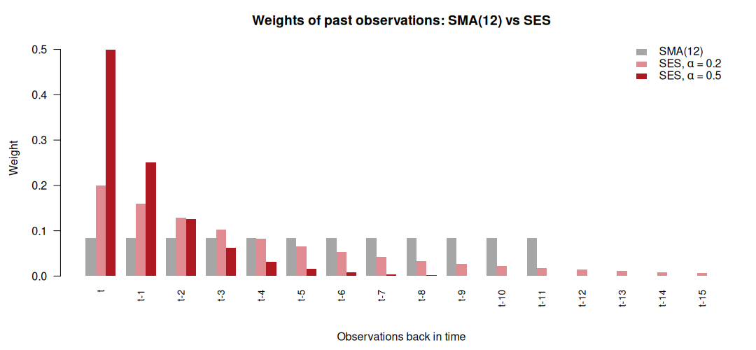
Take \(\alpha=0.5\). The most recent observation gets the weight of 0.5, the one before it 0.5 × 0.5 = 0.25, the one before that 0.5 × 0.5² = 0.125, and so on. The weights decay exponentially. So, instead of 12 parameters, we define just one, and it determines how fast the weights decay. The chart in this post compares the equal weights of SMA(12) with SES for \( \alpha=0.2 \) and \( \alpha=0.5 \): the closer α is to zero, the more evenly the weights are spread; the closer it is to one, the more weight goes to the most recent observation, and the faster the older ones are forgotten.
There are tons of papers discussing SES, its modifications and extensions. Gardner (1985 and 2006) is the best review on the topic. And finally, SES is a predecessor of ETS, and its mechanism is used in TBATS.
How do you choose α in practice, and what do you do when SES is not enough? This is what we discuss in our Demand Forecasting Principles course.